


Physics for the 21st Century
Biophysics Online Textbook
Online Text by Robert Austin
The videos and online textbook units can be used independently. When using both, it is possible to start with either one. Watching the video first, and then reading the unit from the online textbook is recommended.
Each unit was written by a prominent physicist who describes the cutting edge advances in his or her area of research and the potential impacts of those advances on everyday life. The classical physics related to each new topic is covered briefly to help the reader better understand the research, its effects, and our current understanding of physics.
Click on “Content By Unit” (in the menu to the left) and select a unit title to view the Web version of the online text, which includes links to related material. Or, download PDF versions of the units below.
1. Introduction
Biology is complicated, really, really complicated. This should not surprise you if you think that ultimately the laws of physics explain how the world works, because biological activity is far beyond the usual realm of simple physical phenomena. It is easy to simply turn away from a true physical explanation of biological phenomena as simply hopeless. Perhaps it is hopelessly complex at some level of detail. The ghosts of biological “stamp collecting” are still alive and well and for a good reason.

Figure 1: A population of slime-mold cells forms an aggregate in response to a signaling molecule.
Source: © Courtesy of BioMed Central Ltc. From: Maddelena Arigoni et al. “A novel Dictyostelium RasGEF required for chemotaxis and development,” BMC Cell Biology, 7 December 2005.
However, it is possible that in spite of the seemingly hopeless complexity of biology, there are certain emergent properties that arise in ways that we can understand quantitatively. An emergent property is an unexpected collective phenomenon that arises from a system consisting of interacting parts. You could call the phenomenon of life itself an emergent property. Certainly no one would expect to see living systems arise directly from the fundamental laws of quantum mechanics and the Standard Model that have been discussed in the first seven units of this course.
The danger is that this concept of “emergent properties” is just some philosophical musing with no real deeper physics content, and it may be true that the emergent properties of life viewed “bottom up” are simply too complex in origin to understand at a quantitative level. It may not be possible to derive how emergent properties arise from microscopic physics. In his book A Different Universe: Reinventing Physics from the Bottom Down, the physicist Robert Laughlin compares the local movement of air molecules around an airplane wing to the large-scale turbulent hydrodynamic flow of air around the airfoil that gives rise to lift. Molecular motion is clearly the province of microscopic physics and statistical mechanics, while turbulent flow is an emergent effect. As Laughlin puts it, if he were to discover that Boeing Aircraft began worrying about how the movement of air molecules collectively generates hydrodynamics, it would be time to divest himself of Boeing stock. Perhaps the same should have been said when banks started hiring theoretical physicists to run stock trading code.
In biology, we have a much greater problem than with the airplane, because the air molecules can be described pretty well with the elegant ideas of statistical mechanics. So, while it is a long stretch to derive the emergence of turbulence from atomic motion, no one would say it is impossible, just very hard.

Figure 2: Colored smoke marks the hydrodynamic flow around an aircraft, an emergent phenomenon.
Source: © NASA Langley Research Center (NASA-LaRC).
The path of air flowing around the wing of this agricultural aircraft is marked by colored smoke. The large spiral at the tip of the wing, called the “wake vortex,” creates dangerous conditions for a plane flying too close behind. NASA researchers, in conjunction with the FAA, are trying to gain a thorough understanding of wake vortices as part of a program to increase the capacity of crowded airports. They are studying the phenomenon from the bottom up using supercomputer simulations, and from the top down using wind tunnels and flight tests in planes specially equipped for research. (Unit: 9)
In biology, even the fundamentals at the bottom may be impossibly hard for physics to model adequately in the sense of having predictive power to show the pathways of emergent behavior. A classic example is the signaling that coordinates the collective aggregation of the slime-mold Dictyostelium cells in response to the signaling molecule cyclic AMP (cAMP). In the movie shown in Figure 1, the individual Dictyostelium cells signal to each other, and the cells stream to form a fruiting body in an emergent process called “chemotaxis.” This fairly simple-looking yet spectacular process is a favorite of physicists and still not well understood after 100 years of work.
So, perhaps in a foolhardy manner, we will move forward to see how physics, in the discipline known as biological physics, can attack some of the greatest puzzles of them all. We will have to deal with the emergence of collective phenomena from an underlying complex set of interacting entities, like our Dictyostelium cells. But that seems still within the province of physics: really hard, but physics. But there are deeper questions that seem to almost be beyond physics.
Are there emergent physics rules in life?
The amazing array of knowledge in previous units contains little inkling of the complex, varied phenomena of life. Life is an astonishingly emergent property of matter, full-blown in its complexity today, some billions of years after it started out in presumably some very simple form. Although we have many physical ways to describe a living organism, quantifying its state of aliveness using the laws of physics seems a hopeless task. So, all our tools and ideas would seem to fail at the most basic level of describing what life is.
Biology has other incredible emergent behaviors that you can hardly anticipate from what you have learned so far. British physicist Paul Dirac famously said that, “The fundamental laws necessary for the mathematical treatment of a large part of physics and the whole of chemistry are thus completely known, and the difficulty lies only in the fact that application of these laws leads to equations that are too complex to be solved.” Our question is: Is the biological physics of the emergent properties of life simply a matter of impossible complexity, or are there organizing principles that only appear at a higher level than the baseline quantum mechanics?
So far, we have talked about the emergent nature of life itself. The next astonishing emergent behavior we’ll consider is the evolution of living organisms to ever-higher complexity over billions of years. It is strange enough that life developed at all out of inanimate matter, in apparent conflict with the Second Law of Thermodynamics. The original ur-cell, improbable as it is, proceeded to evolve to ever-greater levels of complexity, ultimately arriving at Homo sapiens several million years ago. Thanks to Darwin and Wallace and their concept of selection of the fittest, we have a rather vague hand-waving idea of how this has happened. But the quantitative modeling of evolution as an emergent property remains in its infancy.
The building blocks of evolution

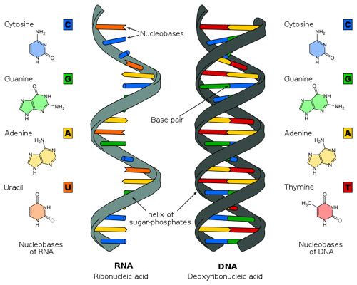
Figure 3: Molecules of life: RNA (left) and DNA (right).
Source: © Wikimedia Commons, Creative Commons Attribution-Share Alike 3.0 license. Author: Sponk, 23 March 2010.
These two molecules, RNA on the left and DNA on the right, form the basis of life as we know it. They have a remarkably simple structure, each being made of a set of four base molecules called nitrogenous bases. The bases of DNA form pairs, which attach to one another and twist into a double helix, while RNA forms a single helix. Biologists can study how DNA replicates and how the instructions contained within its molecular structure are carried out through chemical reactions in a living organism. Predicting the emergent phenomenon of life and how each organism with its own unique features arises from the structure of these molecules is far more difficult. (Unit: 9)Modeling evolution is a difficult task; but nevertheless, we can try. So let’s start at the top and work down. Physicists believe (and it is somewhat more of a belief than a proven fact) that all life began with some ur-cell and that life evolved from that ur-cell into the remarkable complexity of living organisms we have today, including Homo sapiens. We will never know what path this evolution took. But the remarkable unity of life (common genetic code, common basic proteins, and common basic biological pathways) would indicate that, at its core, the phenomenon of life has been locked in to a basic set of physical modes and has not deviated from this basic set. At that core, lies a very long linear polymer, deoxyribonucleic acid (or DNA), which encodes the basic self-assembly information and control information. A related molecule, ribonucleic acid (RNA), has a different chemical group at one particular position, and that profoundly changes the three-dimensional structure that RNA takes in space and its chemical behavior.
Although evolution has played with the information content of DNA, its basic core content, in terms of how its constituent molecules form a string of pairs, has not obviously changed. And while there is a general relationship between the complexity of an organism and the length of its DNA that encodes the complexity, some decidedly simpler organisms than Homo sapiens have considerably longer genomes. So, from an information perspective, we really don’t have any iron-clad way to go from genome to organismal complexity, nor do we understand how the complexity evolved. Ultimately, of course, life is matter. But, it is the evolution of information that really lies at the unknown heart of biological physics, and we can’t avoid it.
The emergence of the mind in living systems

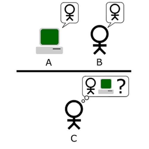
Figure 4: Player C is trying to determine which player—A or B—is a computer and which is human.
Source: © Wikimedia Commons, Public Domain. Author: Bilby, 25 March 2008.
Biology possesses even deeper emergent phenomena than the evolution of complexity. The writer and readers of this document are sentient beings with senses of identity and self and consciousness. Presumably, the laws of physics can explain the emergent behavior of consciousness, which certainly extends down from Homo sapiens into the “lower” forms of life (although those lower forms of life might object to that appellation). Perhaps the hardest and most impossible question in all of biological physics is: What is the physical basis behind consciousness? Unfortunately, that quest quickly veers into the realm of the philosophical and pure speculation; some would say it isn’t even a legitimate physics question at all.
There is even an argument as to whether “machines,” now considered to be computers running a program, will ever be able to show the same kind of intelligence that living systems such as human beings possess. Traditional reductionist physicists, I would imagine, simply view the human mind as some sort of a vastly complicated computational machine. But it is far from clear if this view is correct. The mathematician Alan Turing, not only invented the Turing machine, the grandfather of all computers, but he also asked a curious question: Can machines think? To a physicist, that is a strange question for it implies that maybe the minds of living organisms somehow have emergent properties that are different from what a manmade computing machine could have. The answer to Turing’s question rages on, and that tells us that biology has very deep questions still to be answered.
2. Physics and Life
Here’s a question from a biologist, Don Coffey at Johns Hopkins University: Is a chicken egg in your refrigerator alive? We face a problem right away: What does being alive actually mean from a physics perspective? Nothing. The concept of aliveness has played no role in anything you have been taught yet in this course. It is a perfectly valid biological question; yet physics would seem to have little to say about it. It is an emergent property arising from the laws of physics, which presumably are capable of explaining the physics of the egg.

Figure 5: A chicken egg. Is it alive or dead?
The geometrically elegant, conceptually simple chicken egg presents a challenge to those who want to deduce everything from the laws of physics: How can you determine whether there’s life inside? Although there are straightforward ways to determine that certain things haven’t killed potentially live cells in there, and whether conditions are consistent with cells being alive, it is remarkably difficult to make a positive determination. Physics also has not yet determined which came first, the chicken or the egg. (Unit: 9)
The chicken egg is a thing of elegant geometric beauty. But its form is not critical to its state of aliveness (unless, of course, you smash it). However, you can ask pertinent physical questions about the state of the egg to determine whether it is alive: Has the egg been cooked? It’s pretty easy to tell from a physics perspective: Spin the egg around the short axis of the ellipse rapidly, stop it suddenly, and then let it go. If it starts to spin again, it hasn’t been cooked because the yolk proteins have not been denatured by heat and so remain as a viscous fluid. If your experiment indicates the egg hasn’t been cooked it might be alive, but this biological physics experiment wouldn’t take you much closer to an answer.
Assuming you haven’t already broken the egg, you can now drop it. If you were right that it has not been cooked, the egg will shatter into hundreds of pieces. Is it dead now? If this were your laptop computer, you could pick up all the pieces and—if you are good enough—probably get it working again. However, all of the king’s horses and all the king’s men can’t put Humpty Dumpty back together again and make him alive once more; we don’t know how to do it. The egg’s internal mechanical structure is very complex and rather important to the egg’s future. It, too, is part of being alive, but surely rather ancillary to the main question of aliveness.
Aliveness is probably not a yes-no state of a system with a crisp binary answer, but rather a matter of degree. One qualitative parameter is the extent to which the egg is in thermodynamic equilibrium with its surroundings. If it is even slightly warmer, then I would guess that the egg is fertilized and alive, because it is out of thermodynamic equilibrium and radiating more energy than it absorbs. That would imply that chemical reactions are running inside the egg, maintaining the salt levels, pH, metabolites, signaling molecules, and other factors necessary to ensure that the egg has a future some day as a chicken.
Wait, the egg has a future? No proton has a future unless, as some theories suggest, it eventually decays. But if the egg is not dropped or cooked and is kept at exactly the right temperature for the right time, the miracle of embryonic development will occur: The fertilized nucleus within the egg will self-assemble in an intricate dance of physical forces and eventually put all the right cells into all the right places for a chick to emerge. Can the laws of physics ever hope to predict such complex emergent phenomena?
Emergent and adaptive behavior in bacteria
Here’s an explicit example of what we are trying to say about emergent behavior in biology. Let’s move from the complex egg where the chick embryo may be developing inside to the simple example of bacteria swimming around looking for food. It’s possible that each bacterium follows a principle of every bug for itself: They do not interact with each other and simply try to eat as much food as possible in order to reproduce in an example of Darwinian competition at its most elemental level. But food comes and food goes at the bacterial level; and if there is no food, an individual bacterium will starve and not be able to survive. Thus, we should not be surprised that many bacteria do not exist at the level as rugged individuals but instead show quite startling collective behavior, just like people build churches.
Figure 6: Random motion of gas molecules—bottom up.
Source: © Wikimedia Commons, GNU Free Documentation License. Author: Greg L., 25 August 2006.
If bacteria acted as rugged individuals, then we would expect their movement through space looking for food to resemble what is called a random walk, which is different from the Brownian motion that occurs due to thermal fluctuations. In a random walk there is a characteristic step size L, which is how far the bacterium swims in one direction before it tumbles and goes off randomly in a new direction. Howard Berg at Harvard University has beautiful videos of this random movement of bacteria. The effect of this random motion is that we can view individual bacteria rather like the molecules of a gas, as shown in Figure 6. If that were all there is to bacterial motion, we would be basically done, and we could use the mathematics of the random walk to explain bacterial motion.
However, bacteria can be much more complicated than a gas when viewed collectively. In the Introduction, we discussed the chemotaxis of a population of individual Dictyostelium cells in response to a signal created and received by the collective population of the Dictyostelium cells. Bacteria do the same thing. Under stress, they also begin signaling to each other in various ways, some quite scary. For example, if one bacterium mutates and comes up with a solution to the present problem causing the stress, in a process called “horizontal gene transfer” they secrete the gene and transfer it to their buddies. Another response is to circle the wagons: The bacteria signal to each other and move together to form a complex community called a “biofilm.” Figure 7 shows a dramatic example of the growth of a complex biofilm, which is truly a city of bacteria.

Figure 7: Growth of a biofilm of the bacteria Bacillis subtilisover four days.
Source: © Time-lapse movie by Dr. Remco Kort—published in J. Bacteroi. (2006) 188:3099-109.
The mystery is how the supposedly simple bacteria communicate with each other to form such a complex and adapted structure. There is a set of equations, called the “Keller-Segel equations,” which are usually the first steps in trying to puzzle out emergent behavior in a collection of swimming agents such as bacteria. These equations are not too hard to understand, at least in principle. Basically, they take the random walk we discussed above and add in the generation and response of a chemoattractant molecule. A sobering aspect of these equations is that they are very difficult to solve exactly: They are nonlinear in the density of the bacteria, and one of the great secrets of physics is that we have a very hard time solving nonlinear equations.
Principles of a complex adaptive system
We are just skimming the surface of a monumental problem in biological physics: How agents that communicate with each other and adapt to the structures that they create can be understood. A biological system that communicates and adapts like the film-forming bacteria is an example of a complex adaptive system (CAM). In principle, a complex adaptive system could appear almost anywhere, but biological systems are the most extreme cases of this general phenomenon.

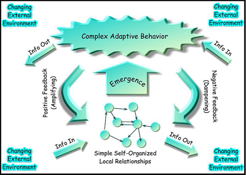
Figure 8: A schematic view of what constitutes a complex adaptive system.
In a complex adaptive system, behavior emerges that is not easily predicted from the component parts of the system and various input stimuli. Information flows into a system in a changing external environment, prompting a response in the form of self-organization. Information flows back into the environment, allowing both positive and negative feedback mechanisms to contribute to the system’s next round of response. In this unit, we consider examples of complex adaptive systems in biology from the molecular level to the behavior of whole organisms, colonies of organisms, and the human brain. A much broader range of systems display this behavior, however, including the stock market and flow of immigrants across the semi-permeable U.S. land border. (Unit: 9)
Source: © Wikimedia Commons, Creative Commons Attribution ShareAlike 3.0.
The computer scientist John Holland and the physicist Murray Gell-Mann, who played a major role in the physics developments you read about in Units 1 through 4, have tried to define what makes a complex adaptive system. We can select a few of the key properties as presented by Peter Freyer that are most germane to biological systems:
- Emergence: We have already discussed this concept, both in this unit and in Unit 8.
- Co-evolution: We will talk about evolution later. Coevolution refers to how the evolution of one agent (say a species, or a virus, or a protein) affects the evolution of another related agent, and vice versa.
- Connectivity: This is concerned with biological networks, which we will discuss later.
- Iteration: As a system grows and evolves, the succeeding generations learn from the previous ones.
- Nested Systems: There are multiple levels of control and feedback.
These properties will appear time and again throughout this unit as we tour various complex adaptive systems in biology, and ask how well we can understand them using the investigative tools of physics.
3. The Emergent Genome
The challenge of biological physics is to find a set of organizing principles or physical laws that governs biological systems. It is natural to start by thinking about DNA, the master molecule of life. This super-molecule that apparently has the code for the enormous complexity seen in living systems is a rather simple molecule, at least in principle. It consists of two strands that wrap around each other in the famous double helix first clearly described by physicist Francis Crick and his biologist colleague James Watson. While the structure of DNA may be simple, understanding how its structure leads to a living organism is not.

Figure 9: The double helix.
Source: © Wikimedia Commons, Public Domain. Author: brian0918, 22 November 2009.
We will use the word “emergent” here to discuss the genome in the following sense: If DNA simply had the codes for genes that are expressed in the organism, it would be a rather boring large table of data. But there is much more to the story than this: Simply knowing the list of genes does not explain the implicit emergence of the organism from this list. Not all the genes are expressed at one time. There is an intricate program that expresses genes as a function of time and space as the organism develops. How this is controlled and manipulated still remains a great mystery.
As Figure 9 shows, the DNA molecule has a helicity, or twist, which arises from the fundamental handedness, or chirality, of biologically derived molecules. This handedness is preserved by the fact that the proteins that catalyze the chemical reactions are themselves handed and highly specific in preserving the symmetry of the molecules upon which they act. The ultimate origin of this handedness is a controversial issue. But we assume that a right-handed or left-handed world would work equally well, and that chiral symmetry breaking such as what we encountered in Unit 2 on the scale of fundamental particles is not present in these macroscopic biological molecules.
It is, however, a mistake to think that biological molecules have only one possible structure, or that somehow the right-handed form of the DNA double helix is the only kind of helix that DNA can form. It turns out that under certain salt conditions, DNA can form a left-handed double helix, as shown in Figure 10. In general, proteins are built out of molecules called “amino acids.” DNA contains the instructions for constructing many different proteins that are built from approximately 20 different amino acids. We will learn more about this later, when we discuss proteins. For now, we will stick to DNA, which is made of only four building blocks: the nitrogenous bases adenine (A), guanine (G), cytosine (C), and thymine (T). Adenine and guanine have a two-ring structure, and are classified as purines, while cytosine and thymine have a one-ring structure and are classified as pyrimidines. It was the genius of Watson and Crick to understand that the basic rules of stereochemistry enabled a structure in which the adenine (purine) interacts electrostatically with thymine (pyrimidine), and guanine (purine) interacts with cytosine (pyrimidine) under the salt and pH conditions that exist in most biological systems.

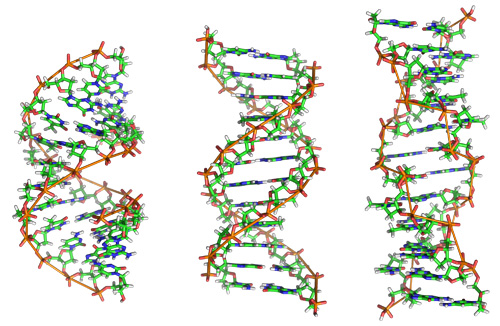
Figure 10: The DNA double helix, in three of its possible configurations.
While the DNA double helix most often appears as the right-handed helix shown in Figure 9, it can take on many different configurations. Here, we see A-DNA (left), B-DNA (center), and Z-DNA (right). B-DNA is the configuration most often found in living cells. A-DNA forms a wider spiral. DNA takes this form in the partially dehydrated samples sometimes studied in the laboratory. Z-DNA is a left-handed double helix with a zig-zag structure not seen in B-DNA. These three configurations are all biologically active and both the B- and Z- configurations have been found in living cells. Which form the molecule takes depends primarily on the level of hydration in the environment surrounding the molecule, and what ions and other organic compounds are present. (Unit: 9)
Source: © Wikimedia Commons, GNU Free Documentation License, Version 1.2. Author: Zephyris (Richard Wheeler), 4 February 2007.
Not only does the single-stranded DNA (ssDNA) molecule like to form a double-stranded (dsDNA) complex, but the forces that bring the two strands together result in remarkably specific pairings of the base pairs: A with T, and G with C. The pyrimidine thymine base can form strong electrostatic links with the purine adenine base at two locations, while the (somewhat stronger) guanine-cytosine pair relies on three possible hydrogen bonds. The base pairs code for the construction of the organism. Since there are only bases in the DNA molecule, and there are about 20 different amino acids, the minimum number of bases that can uniquely code for an amino acid is three. This is called the triplet codon.
The remarkable specificity of molecular interactions in biology is actually a common and all-important theme. It is also a physics problem: How well do we have to understand the potentials of molecular interactions before we can begin to predict the structures that form? We will discuss this vexing problem a bit more in the protein section, but it remains a huge problem in biological physics. At present, we really cannot predict three-dimensional structures for biological structures, and it isn’t clear if we ever will be able to given how sensitive the structures are to interaction energies and how complex they are.
An example of this extreme sensitivity to the potential functions and the composition of the polymer can be found in the difference between ribonucleic acids (RNA) and deoxyribonucleic acids (DNA). Structurally, the only difference between RNA and DNA is that at the 2′ position of the ribose sugar, RNA has a hydroxyl (OH) molecule—a molecule with one hydrogen and one oxygen atom—while DNA just has a hydrogen atom. Figure 11 shows what looks like the completely innocuous difference between the two fundamental units. From a physicist’s bottom-up approach and lacking much knowledge of physical chemistry, how much difference can that lone oxygen atom matter?

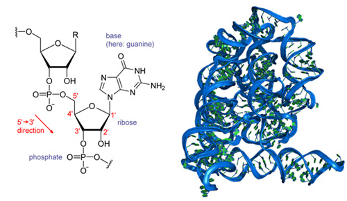
Figure 11: The chemical structure of RNA (left), and the form the folded molecule takes (right).
Source: © Left: Wikimedia Commons, Public Domain. Author: Narayanese, 27 December 2007. Right: Wikimedia Commons, Public Domain. Author: MirankerAD, 18 December 2009.
The chemical structure of RNA, like that of DNA, is relatively simple. On the left, we see a diagram of a portion of the RNA molecule that highlights its difference from DNA. RNA has a hydroxyl (OH) molecule—a molecule with one hyrogen and one oxygen atom—at the 2′ position on the ribose sugar, where DNA has a hydrogen atom. The result of this seemingly innocuous swap is shown on the right: RNA folds into structures that are far more complex than the DNA double helix. (Unit: 9)
Unfortunately for the bottom-up physicist, the news is very bad. RNA molecules fold into a far more complex structure than DNA molecules do, even through the “alphabet,” for the structures are just four letters: A,C, G, and bizarrely U, a uracil group that Nature for some reason has favored over the thymine group of DNA. An example of the complex structures that RNA molecules can form is shown in Figure 11. Although the folding rules for RNA are vastly simpler than those for DNA, we still cannot predict with certainty the three-dimensional structure an RNA molecule will form if we are given the sequence of bases as a starting point.
The puzzle of packing DNA: chromosomes
Let’s consider a simpler problem than RNA folding: packaging DNA in the cell. A gene is the section of DNA that codes for a particular protein. Since an organism like the bacterium Escherichia coli contains roughly 4,000 different proteins and each protein is roughly 100 amino acids long, we would estimate that the length of DNA in E. coli must be about 2 million base pairs long. In fact, sequencing shows that the E. coli genome actually consists of 4,639,221 base pairs, so we are off by about a factor of two, not too bad. Still, this is an extraordinarily long molecule. If stretched out, it would be 1.2 mm in length, while the organism itself is only about 1 micron long.
The mathematics of how DNA actually gets packaged into small places, and how this highly packaged polymer gets read by proteins such as RNA polymerases or copied by DNA polymerases, is a fascinating exercise in topology. Those of you who are fishermen and have ever confronted a highly tangled fishing line can appreciate that the packaging of DNA in the cell is a very nontrivial problem.
The physics aspect to this problem is the stiffness of the double helix, and how the topology of the twisted and folded molecule affects its biological function. How much energy does it take to bend or twist the polymer into the complex shapes necessary for efficient packaging of DNA in a cell? And how does the intrinsic twist of the double helix translate into the necessity to break the double helix and reconnect it when the code is read by proteins? In other words, biological physics is concerned with the energetics of bending DNA and the topological issues of how the DNA wraps around in space.
The incredible length of a DNA molecule, already bad enough for bacteria, gets more outrageous for higher organisms. Most mammals have roughly 3 x 10⁹ base pairs wrapped up into chromosomes, which are very complex structures consisting of proteins and nucleic acids. However, although we view ourselves as being at the peak of the evolutionary ladder, there seems to be much more DNA in organisms we view as our intellectual inferiors: Some plants and amphibians have up to 1011 base pairs! If we laid out the DNA from our chromosomes in a line, it would have a length of approximately 1 meter; that of amphibians would stretch over 30 meters!
Dark matter in the genome
Why is the human DNA genome so long, and other genomes even longer still? We don’t know exactly how many genes the human genome contains, but a reasonable guess seems to indicate about 30,000. If we imagine that each gene codes for a protein that has about 100 amino acids, and that three base pairs are required to specify each amino acid, the minimal size of the human genome would be about 107 base pairs. It would seem that we have at least 1,000 times as much DNA as is necessary for coding the genome. Clearly, the amount of “excess” DNA must be much higher for plants and amphibians. Apparently, the DNA is not efficiently coded in the cell, in the sense that lots of so-called “junk” DNA floats around in a chromosome. In fact, a large amount of noncoding DNA has a repeating motif. Despite some guesses about what role this DNA plays, its function remains a substantial puzzle. Perhaps the information content of the genome is not just the number of base pairs, but that there is much “hidden” information contained in this dark genome.
We have succeeded in sequencing the coding part of the human genome, but not the dark part. Are we done now that we know the coding sequence of one given individual? Hardly. We don’t know how to extract the information content of the genome at many levels, or even how to define the genome’s information quantitatively. The concept of “information” is not only a tricky concept, but also of immense importance in biological physics. Information is itself an emergent property in biology, and it is contextual: The environment gives meaning to the information, and the information itself means little without the context of the environment.
One problem is that we don’t know how to measure information in the genome. Paradoxically, information to a physicist is related to entropy, which is a quantitative measure of disorder. The lower the entropy, the higher the information content. We do, however, need to be careful how we define entropy, because the standard equation in undergraduate physics courses does not apply to a string of base pairs.
Different meanings of information

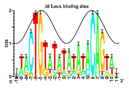
Figure 12: This sequence logo is a compact way of displaying information contained in a piece of genetic material.
Source: © P. P. Papp, D. K. Chattoraj, and T. D. Schneider, Information Analysis of Sequences that Bind the Replication Initiator RepA, J. Mol. Biol., 233, 219-230, 1993.
This sequence logo represents how often each base pair appears at each position in a genetic sequence with the relative height of the letters, while the total height of a stack of letters represents the information content of that position in units of bits. The logo is a compact, easy-to-read summary of genetic information. (Unit: 9)
The introduction of entropy emphasizes a critical point: Information has a different meaning to a biologist than it does to a physicist. Suppose you look at some stretch of the genome, and you find that all four of the bases are present in roughly equal numbers—that is, a given base pair has a 25 percent chance to be present in the chain. To a biologist, this implies the sequence is coding for a protein and is information-rich. But a physicist would say it has high entropy and low information, somewhat like saying that it may or may not rain tomorrow. If you say it will rain tomorrow, you convey a lot of information and very little obvious entropy. The opposite is true in gene sequences. To a biologist, a long string of adenines, AAAAAAAAAAAA, is useless and conveys very little information; but in the physics definition of entropy, this is a very low entropy state. Obviously, the statistical concepts of entropy and the biological concepts of information density are rather different.
The dark matter that makes up a huge fraction of the total genome is still very much terra incognito. Entropy density maps indicate that it has a lower information density (in the biologist’s use of the word) than the “bright matter” coding DNA. Unraveling the mysteries of the dark matter in the genome will challenge biologists just as much as exploring the cosmological variety challenges astrophysicists.
4. Proteins
Having explored the emergent genome in the form of DNA from a structural and informational perspective, we now move on to the globular polymers called “proteins,” the real molecular machines that make things tick. These proteins are the polymers that the DNA codes and are the business end of life. They regulate the highly specific chemical reactions that allow living organisms to live. At 300 K (80°F), the approximate temperature of most living organisms, life processes are characterized by tightly controlled, highly specific chemical reactions that take place at a very high rate. In nonliving matter, highly specific reactions tend to proceed extremely slowly. This slow reaction rate is another result of entropy, since going to a highly specific reaction out of many possible reactions is extremely unlikely. In living systems, these reactions proceed much faster because they are catalyzed by biological proteins called enzymes. It is the catalysis of very unlikely chemical reactions that is the hallmark of living systems.

Figure 13: The enzyme on the left has a much easier time reading DNA than the enzyme on the right due to structural details that are difficult to predict from first principles.
Source: © RCSB Protein Data Bank
The mystery of how these protein polymers do their magical chemical catalysis is basically the domain of chemistry, and we won’t pursue it further here. As physicists, we will turn our attention to the emergent structure of biological molecules. We saw in the previous section how DNA, and its cousin RNA, have a relatively simple structure that leads, ultimately, to the most complex phenomena around. In this section, we will ask whether we can use the principles of physics to understand anything about how the folded structure of proteins, which is incredibly detailed and specific to biological processes, arises from their relatively simple chemical composition.
Proteins: the emergence of order from sequence
As polymers go, most proteins are relatively small but much bigger than you might expect is necessary. A typical protein consists of about 100 to 200 monomer links; larger polymers are typically constructed of subunits consisting of smaller balls of single chains. For example, the protein RNA polymerase, which binds to DNA and creates the single-strand polymer RNA, consists (in E. coli) of a huge protein with about 500,000 times the mass of a hydrogen atom, divided into five subunits. Despite their small size, folded proteins form exceedingly complex structures. This complexity originates from the large number of monomer units from which the polymers are formed: There are 21 different amino acids. We saw that RNA could form quite complex structures from a choice of four different bases. Imagine the complexity of the structures that can be formed in a protein if you are working with a choice of 21 of them.

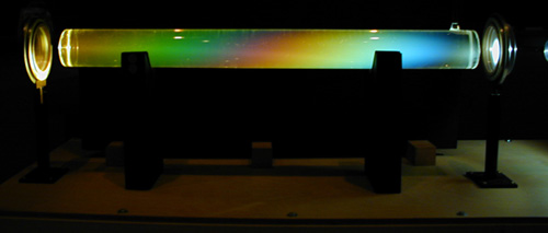
Figure 14: As polarized light passes through corn syrup, which is full of right-handed sugar molecules, its plane of polarization is rotated.
Source: © Technical Services Group, MIT Department of Physics.
This tube of corn syrup is filled with right-handed sugar molecules. As polarized white light passes through the tube, its plane of polarization is rotated by an amount that depends on the wavelength, or color, of the light. The result is the rainbow shown here. (Unit: 9)
Note that you can assign a handedness to the bonding pattern within the protein: Some proteins are left-handed, and others are right-handed. Experimentally, it was observed that naturally occurring biological molecules (as opposed to molecules synthesized in the laboratory) could rotate the plane of polarization of light when a beam of light is passed through a solution of the molecule. It is easy to see this by getting some maple syrup from a store and observing what happens when a polarized laser beam passes through it. First, orient an “analyzing” polarizer so that no laser light passes through it. Then put the syrup in the laser’s path before the analyzing polarizer. You will notice that some light now passes through the polarizer. The beam polarization (as you look at it propagating toward you) has rotated counterclockwise, or in a right-handed sense using the right-hand rule. The notation is that the sugar in the syrup is dextro-rotary (D-rotary), or right-handed. In the case of the amino acids, all but one are left-handed, or L-rotary. Glycine is the one exception. It has mirror symmetry.
We know how to denote the three-dimensional structure of a protein in a rather concise graphical form. But when you actually see the space-filling picture of a protein—what it would look like if you could see something that small—your physicist’s heart must stop in horror. It looks like an ungodly tangled ball. Who in their right mind could possibly be interested in this unkempt beast?

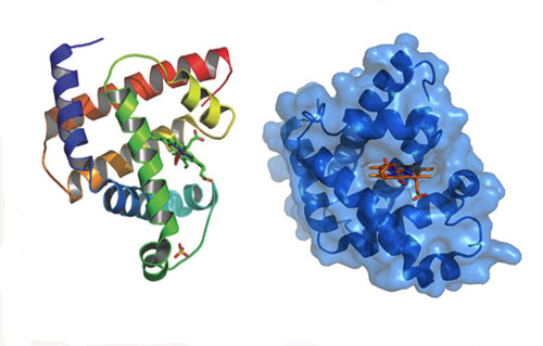
Figure 15: The structure of myoglobin (left) and the form it actually takes in space (right).
Source: © Left: Wikimedia Commons, Public Domain. Author: AzaToth, 27 February 2008; right: Wikimedia Commons Creative Commons Attribution-Share Alike 3.0 Unported License. Author: Thomas Splettstoesser, 10 July 200
Here, we see two drawings of the myoglobin molecule that binds to iron and oxygen in muscle tissue. The iron bound to myoglobin is what gives meat its red color. The iron is bound to a central ring structure, which is surrounded by a long chain of amino acids that fold around the central ring in a series of helices. The drawing on the left is an accurate sketch of the ring surrounded by helices. On the right, we see what this molecule looks like in a space-filling diagram: a very complicated blob. (Unit: 9)
We can say some general things about protein structure. First, the nearest-neighbor interactions are not totally random; they often show a fair amount of order. Experiments have revealed that nature uses several “motifs” in forming a globular protein, roughly specified by the choice of amino acids which naturally combine to form a structure of interest. These structures, determined primarily by nearest-neighbor interactions, are called “secondary structures.” We commonly see three basic secondary structures: the  -helix, the
  -strand (these combine into sheets), and the polyproline helix.
We can now begin to roughly build up protein structures, using the secondary structures as building blocks. For example, one of my favorite proteins is myoglobin because it is supposed to be simple. It is not. We can view it as basically a construction of several alpha helices which surround a “prosthetic group,” the highly conjugated heme structure used extensively in biology. Biologists often regard myoglobin as a simple protein. One possible function is to bind oxygen tightly as a storage reservoir in muscle cells. There may be much more to this molecule than meets the eye, however.
As their name indicates, globular proteins are rather spherical in shape. Also, the polarizability of the various amino acids covers quite a large range, and the protein is designed (unless it is membrane-bound) to exist in water, which is highly polar. As biologists see it, the polarizable amino acids are predominantly found in the outer layer of the globular protein, while the non-polar amino acids reside deep in the interior. This arrangement is not because the non-polar amino acids have a strong attraction for one another, but rather because the polar amino acids have strong interactions with water (the so-called hydrophilic effect) and because introducing non-polar residues into water gives rise to a large negative entropy change (the so-called hydrophobic effect). So, physics gives us some insight into structure, through electrostatic interactions and entropy.

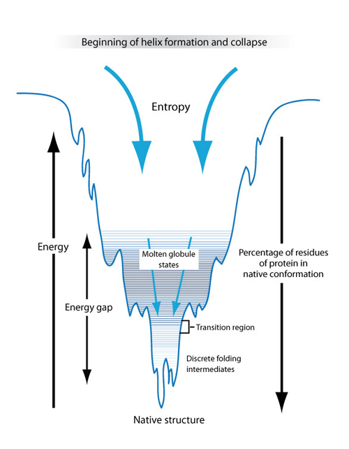
Figure 16: A schematic of how minimizing the free energy of a molecule could lead to protein folding.
The above diagram sketches one possible explanation for how proteins fold into their native structures that is based on the physics concept of minimizing free energy. In this model, the unfolded protein had both high entropy and high free energy. The high entropy corresponds to there being a large number of possible conformational states—the molecule can take on many different three-dimensional shapes. The high free energy means that the molecule is unstable, and flops easily between the different conformational states. As the protein starts to fold, the free energy drops and the number of available conformational states (denoted by the width of the funnel) decreases. There are local minima along the way that can trap the protein in a metastable state for some time, slowing its progress towards the free energy minimum. At the bottom of the funnel, the free energy is at a minimum and there is only one conformational state available to the protein molecule. This is called its native state, and is the ground state of the system. It is possible that the native state is not unique—there can be several states with approximately equal free energy at the bottom of the funnel. (Unit: 9)
One kind of emergence we wish to stress here is that, although you would think that a polymer consisting of potentially 21 different amino acids for each position would form some sort of a glue-ball, it doesn’t. Many proteins in solution seem to fold into rather well-defined three-dimensional shapes. But can we predict these shapes from the amino acid sequence? This question is known as the “protein-folding problem,” and has occupied many physicists over the past 30 some years as they attempt with ever-increasingly powerful computers to solve it. While Peter Wolynes and Jose Onuchich have been able to sketch out some powerful ideas about the general path of the protein folding that make use of the physics concept of free energy, it could well be that solving the puzzle to a precise answer may be impossible.
There may well be a fundamental reason why a precise answer to the folding problem is impossible: because in fact there may be no precise answer! Experiments by Hans Frauenfelder have shown that even for a relatively simple protein like the myoglobin presented in Figure 16, there is not a unique ground state representing a single free energy minimum but rather a distribution of ground states with the same energy, also known as aconformation distribution, which are thermally accessible at 300 K. It is becoming clear that this distribution of states is of supreme importance in protein function, and that the distribution of conformations can be quite extreme; the “landscape” of conformations can be extremely rugged; and within a given local valley, the protein cannot easily move over the landscape to another state. Because of this rugged landscape, a protein might often be found inmetastable states: trapped in a low-lying state that is low, but not the lowest, unable to reach the true ground state without climbing over a large energy barrier.

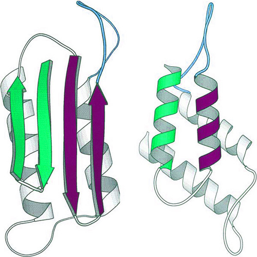
Figure 17: Two possible conformations of a prion protein: on the left as a beta sheet; on the right as an alpha helix.
Source: © Flickr, Creative Commons License. Author: AJC1, 18 April 2007.
Prions, familiar from their role in mad cow disease, can take on two rather different conformations. The prion on the right, in a helical conformation, dissolves easily in water and is relatively benign. The prion on the left, in a beta-sheet conformation, tends to stick to other similar prions and forms plaques. These plaques disrupt the structure of healthy tissue, resulting in the “spongy” texture found in the brains of infected animals. (Unit: 9)
An extreme example of this inherent metastability of many protein structures, and the implication to biology, is the class of proteins called “prions.” These proteins can fold into two different deep valleys of free energy: as an alpha-helix protein rather like myoglobin, or as a beta-sheet protein. In the alpha-helix conformation, the prion is highly soluble in water; but in the beta-sheet conformation, it tends to aggregate and drop out of solution, forming what are called “amyloid plaques,” which are involved with certain forms of dementia. One energy valley leads to a structure that leads to untreatable disease; the other is mostly harmless.
The apparent extreme roughness of biological landscapes, and the problems of ascertaining dynamics on such landscapes, will be one of the fundamental challenges for biological physics and the subject of the next section.
5. Free Energy Landscapes
A certified unsolved problem in physics is why the fundamental physical constants have the values they do. One of the more radical ideas that has been put forward is that there is no deeper meaning. The numbers are what they are because an unaccountable number of alternate universes are forming a landscape of physical constants. We just happen to be in a particular universe where the physical constants have values conducive to form life and eventually evolve organisms who ask such a question.
This idea of a landscape of different universes actually came from biology, evolution theory, in fact, and was first applied to physics by Lee Smolin. Biology inherently deals with landscapes because the biological entities, whether they are molecules, cells, organisms, or ecologies, are inherently heterogeneous and complex. Trying to organize this complexity in a systematic way is beyond challenging. As you saw in our earlier discussion of the protein folding problem, it is easiest to view the folding process as movement on a free energy surface, a landscape of conformations.
Glasses, spin glasses, landscapes
There is a physical system in condensed matter physics that might provide a simpler example of the kind of landscape complexity that is characteristic of biological systems. Glasses are surprisingly interesting physical systems that do not go directly to the lowest free energy state as they cool. Instead, they remain frozen in a very high entropy state. For a physical glass like the windows of your house, the hand-waving explanation for this refusal to crystallize is that the viscosity becomes so large as the system cools, that there is not enough time in the history of the universe to reach the true ground state.

Figure 18: As a glass cools, the viscosity increases so rapidly that the atoms get frozen in a disordered state.
Source: © OHM Equipment, LLC.
Although the glass in your windows may look as clear as a crystal of quartz or sapphire, its structure is radically different. Crystals have a regular, rigid structure on the atomic scale, while glasses at room temperature are messy collections of molecules that flow like an extremely viscous liquid. As glass that has been heated in an oven like the one shown here cools, its viscosity increases dramatically, leaving it stuck far from its ground state in what appears to be a stable solid form. (Unit: 9)
A more interesting glass, and one more directly connected to biology, is the spin glass. It actually has no single ground state, which may be true for many proteins as well. The study of spin glasses in condensed matter physics naturally brings in the concepts of rough energy landscapes, similar to those we discussed in the previous section. The energy landscape of a spin glass is modified by interactions within the material. These interactions can be both random and frustrated, an important concept that we will introduce shortly. By drawing an analogy between spin glasses and biological systems, we can establish some overriding principles to help us understand these complex biological structures.
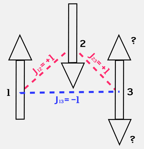
A spin glass is nothing more than a set of spins that interact with each other in a certain way. At the simplest level, a given spin can be pointing either up or down, as we saw in Unit 6; the interaction between two spins depends on their relative orientation. The interaction term Jij specifies how spin i interacts with spin j. Magically, it is possible to arrange the interaction terms between the spins so that the system has a large set of almost equal energy levels, rather than one unique ground state. This phenomenon is called “frustration.”

Figure 19: This simple system of three spins is frustrated, and has no clear ground state.
If the interaction energy between two spins is +1 if they point in the same direction, and -1 if they point in opposite directions, then this very simple spin system is frustrated. Spin 1 points up and spin 2 points down, so their interaction energy is -1. Spin 3 can point either up or down. If it points up, its interaction energy with spin 1 is +1 and its interaction with spin 2 is -1. If it points down, the opposite is true. So spin 3 is frustrated, and the simple rule for choosing a direction based on the lowest energy configuration does not help it pick a direction in which to point. (Unit: 9)
For a model spin glass, the rule that leads to frustration is very simple. We simply set the interaction term to be +1 if the two spins point in the same direction, and -1 if they point in different directions. If you go around a closed path in a given arrangement of spins and multiply all the interaction terms together, you will find that if the number is +1, the spins have a unique ground state; and if it is -1, they do not. Figure 19 shows an example of a simple three-spin system that is frustrated. The third spin has contradictory commands to point up and point down. What to do? Note that this kind of a glass is different from the glass in your windows, which would find the true ground state if it just had the time. The spin glass has no ground state, and this is an emergent property.
Frustration arises when there are competing interactions of opposite signs at a site, and implies that there is no global ground energy state but rather a large number of states with nearly the same energy separated by large energy barriers. As an aside, we should note that this is not the first time we’ve encountered a system with no unique ground state. In Unit 2, systems with spontaneously broken symmetry also had many possible ground states. The difference here is that the ground states of the system with broken symmetry were all connected in field space—on the energy landscape, they are all in the same valley—whereas the nearly equal energy levels in a frustrated system are all isolated in separate valleys with big mountains in between them. The central concept of frustration is extremely important in understanding why a spin glass forms a disordered state at low temperatures, and must play a crucial role in the protein problem as well.
Hierarchical states

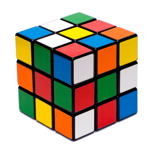
Figure 20: A Rubik’s Cube is a familiar example of a hierarchical distribution of states.
Source: © Wikimedia Commons, GNU Free Documentation License 1.2. Author: Lars Karlsson (Keqs), 5 January 2007.
When you take a new Rubik’s Cube out of the box, it is in a highly ordered state. However, it doesn’t take long before it is in a highly disordered state, with colored squares seemingly randomly distributed. It is very easy to go from one apparently random state to another, but not so easy to find the path through all the possible states that leads back to the original configuration. This is a hierarchical distribution of states not unlike the states available to an unraveled protein molecule trying to fold into its optimal shape. (Unit: 9)
Take a look at a Rubik’s cube. Suppose you have some random color distribution, and you’d like to go back to the ordered color state. If you could arbitrarily turn any of the colored squares, going back to the desired state would be trivial and exponentially quick. However, the construction of the cube creates large energy barriers between states that are not “close” to the one you are in; you must pass through many of the allowed states in some very slow process in order to arrive where you want to be. This distribution of allowed states that are close in “distance” and forbidden states separated by a large distance is called a hierarchical distribution of states. In biology, this distance can mean many things: how close two configurations of a protein are to each other, or in evolution how far two species are apart on the evolutionary tree. It is a powerful idea, and it came from physics.
To learn anything useful about a hierarchy, you must have some quantitative way to characterize the difference between states in the hierarchy. In a spin glass, we can do this by calculating the overlap between two states, counting up the number of spins that are pointing the same way, and dividing by the total number of spins. States that are similar to one another will have an overlap close to one, while those that are very different will have a value near zero. We can then define the “distance” between two states as one divided by the overlap; so states that are identical are separated by one unit of distance, and states that are completely different are infinitely far apart.

Figure 21: Here, we see two possible paths across an energy landscape strewn with local minima.
The movement of a spin glass towards its lowest energy configuration can be represented as movement across a landscape, where the energy of each configuration is represented by the height of the terrain. Here, we see a landscape with the energy continuously decreasing along the x-axis, but there are many low-energy holes of varying depth all over the place. The red and the green lines show two possible paths toward the lowest energy state. Both paths pass through several local minima, from which the system would have needed an energy kick from somewhere to escape. Note the similarity of this landscape to the string landscape in Figure 29 of Unit 4. This similarity is no coincidence. (Unit: 9)
Knowing that the states of a spin glass form a hierarchy, we can ask what mathematical and biological consequences this hierarchy has. Suppose we ask how to pass from one spin state to another. Since the spins interact with one another, with attendant frustration “clashes” occurring between certain configurations, the process of randomly flipping the spins hoping to blunder into the desired final state is likely to be stymied by the high-energy barriers between some of the possible intermediate states. A consistent and logical approach would be to work through the hierarchical tree of states from one state to another. In this way, one always goes through states that are closely related to one another and hence presumably travels over minimum energy routes. This travel over the space is movement over a landscape. In Figure 21, we show a simulated landscape, two different ways that system might pick its way down the landscape, and the local traps which can serve as metastable sticking points.
In some respects, this landscape picture of system dynamics is more descriptive than useful to the central problems in biological physics that we are discussing in this course. For example, in the protein section, we showed the staggering complexity of the multiple-component molecular machines that facilitate the chemical reactions taking place within our bodies, keeping us alive. The landscape movement we have described so far is driven by pre-existing gradients in free energy, not the time-dependent movement of large components. We believe that what we observe there is the result of billions of years of evolution and the output of complex biological networks.
6. Evolution
Biological evolution remains one of the most contentious fields to the general public, and a dramatic example of emergent phenomena. We have been discussing the remarkable complexity of biology, and it is now natural to ask: How did this incredible complexity emerge on our planet? Perhaps a quote from French Nobel Laureate biologist Jacques Monod can put things into perspective: “Darwin’s theory of evolution was the most important theory ever formulated because of its tremendous philosophical, ideological, and political implications.” Today, over 150 years after the publication of “On the Origin of the Species,” evolution remains hotly debated around the world, but not by most scientists. Even amongst the educated lay audience, except for some cranks, few have doubt about Newton’s laws of motion or Einstein’s theories of special and general relativity, but about half of the American public don’t agree with Darwin’s theory of evolution. Surely, physics should be able to clear this up to everybody’s satisfaction.

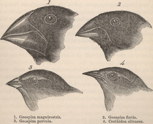
Figure 22: The variation in Galapagos finches inspired Charles Darwin’s thinking on evolution, but may evolve too fast for his theory.
Source: © Public Domain from The Zoology of the Voyage of H.M.S. Beagle, by John Gould. Edited and superintended by Charles Darwin. London: Smith Elder and Co., 1838.
The birds sketched here showcase the diversity of the Galapagos finch population. The finch in the lower left corner lives in trees and eats insects. The one pictured to its right was mistaken for a warbler by Darwin. The top two finches live on the ground and use their heavy beaks to crush the seeds they eat. These finches seem to have evolved from a common ancestor in response to different environmental conditions they encountered on the Galapagos Islands. More recent research, however, indicates that the finch population evolves more quickly to environmental change than can be explained by random mutations. (Unit: 9)
Or maybe not. The problem is that simple theories of Darwinian evolution via random mutations and natural selection give rise to very slow change. Under laboratory conditions, mutations appear at the low rate of one mutated base pair per billion base pairs per generation. Given this low observed rate of mutations, it becomes somewhat problematic to envision evolution via natural selection moving forward to complex organisms such as humans. This became clear as evolution theories tried to move from Darwin’s vague and descriptive anecdotes to a firmer mathematical foundation.
Recent work on the Galapagos Islands by the Princeton University biologists Peter and Rosemary Grant revealed something far more startling than the slow evolution of beak sizes. The Grants caught and banded thousands of finches and traced their elaborate lineage, enabling them to document the changes that individual species make in reaction to the environment. During prolonged drought, for instance, beaks may become longer and sharper, to reach the tiniest of seeds. Here is the problem: We are talking about thousands of birds, not millions. We are talking about beaks that change over periods of years, not thousands of years. How can evolution proceed so quickly?
Fitness landscapes and evolution
In our protein section, we discussed the concept of a free energy landscape. This indicates that proteins do not sit quietly in a single free energy minimum, but instead bounce around on a rough landscape of multiple local minima of different biological functional forms. But this idea of a complex energy landscape did not originate from proteins or spin glasses. It actually came from an American mathematical biologist named Sewall Wright who was trying to understand quantitatively how Darwinian evolution could give rise to higher complexity—exactly the problem that has vexed so many people.

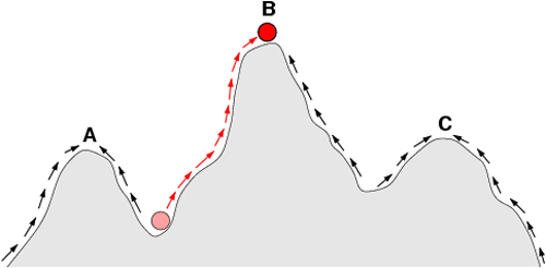
Figure 23: Natural selection can be viewed as movement on a fitness landscape.
Source: © Wikimedia Commons, Public Domain. Author: Wilke, 18 July 2004.
The fitness landscape shown here looks like a slice through the free energy landscape shown in Figure 22, and like an extension of the potential sketched in Figure 25 (Unit 4). These different landscapes are illustrations of the same basic idea in physics: A system seeks its lowest energy state and may have to travel over some energy barriers to get there. Sewall Wright’s fitness landscape illustrates a similar concept, but in reverse. The height of each peak represents the fitness of a given species to survive in a given set of conditions. Selection pressure drives species up to mountain summits in the fitness landscape. Not surprisingly, physicists working on these problems sometimes choose to draw the fitness landscape upside-down. (Unit: 9)
We can put the problem into simple mathematical form. Darwinian evolution is typically believed to be due to the random mutation of genes, which occurs at some very small rate of approximately 10-9 mutations/base pair-generation under laboratory conditions. At this rate, a given base pair would undergo a random mutation every billion generations or so. We also believe that the selection pressure—a quantitative measure of the environmental conditions driving evolution—is very small if we are dealing with a highly optimized genome. The number of mutations that “fix,” or are selected to enter the genome, is proportional to the mutation rate times the selection pressure. Thus, the number of “fixed” mutations is very small. A Galapagos finch, a highly evolved creature with a genome optimized for its environment, should not be evolving nearly as rapidly as it does by this formulation.
There is nothing wrong with Darwin’s original idea of natural selection. What is wrong is our assumption that the mutation rate is fixed at 10-9 mutations/base-pair generation, and more controversially perhaps that the mutations occur at random on the genome, or that evolution proceeds by the accumulation of single base-pair mutations: Perhaps genomic rearrangements and basepair chemical modifications (a process called “epigenetics”) are just as important. Further, we are beginning to understand the role of ecological complexity and the size of the populations. The simple fitness landscape of Figure 23 is a vast and misleading simplification. Even in the 1930s, Seawall Wright realized that the dynamics of evolution had to take into account rough fitness landscapes and multiple populations weakly interbreeding across a rough landscape. Figure 24 dating all the way back to 1932, is a remarkably prescient view of where evolution biological physics is heading in the 21st century.

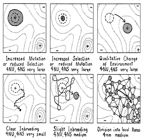
Figure 24: Sewall Wright sketched the path different populations might take on the fitness landscape.
Source: © Sewall Wright, “The Role of Mutation, Inbreeding, Crossbreeding, and Selection in Evolution,” Sixth International Congress of Genetics, Brooklyn, NY: Brooklyn Botanical Garden, 1932.
Sewall Wright, in this 1932 drawing, considered the path different populations might take across the fitness landscape through random mutations and selection pressure. For effective evolution to take place, the population must be able to move from a lower peak to a higher one by moving across a saddle where the level of fitness is lower. In each case, the dashed line represents the initial population sitting on a peak (not necessarily the highest) in the fitness landscape. The shaded area is where the population ends up through natural selection. The top row shows the fate of populations so large that individual mutations have little effect on the whole. In the upper left, the mutation rate is high and the selection pressure is weak, so the population meanders around the fitness hilltop. In the top center, the population concentrates at the fitness peak after living under unchanging conditions for a long time with either a low mutation rate or high selection pressure. In the top right, the environment suddenly changes and the population slowly works its way to a new fitness peak. The lower row shows the fate of smaller populations. In the lower left, a population small enough to be affected by virtually every mutation meanders across the landscape in random steps. In the bottom center, the small population is affected nearly equally by mutations and selection pressure, and easily escapes small peaks while moving very slowly up higher ones. The lower right shows the conditions Wright considered optimal: many small, isolated populations that occasionally interact. These groups can change quickly, but are spared the uncontrolled random wandering of a single small group by virtue of their interaction with one another. (Unit: 9)
Darwinian evolution in a broader sense is also changing the face of physics as the fundamental concepts flow from biology to physics. Darwinian evolution as modified by recent theories teaches us that it is possible to come to local maxima in fitness in relatively short time frames through the use of deliberate error production and then natural selection amongst the errors (mutants) created. This seems somewhat counterintuitive, but the emergence of complexity from a few simple rules and the deliberate generation of mistakes can be powerfully applied to seemingly intractable problems in computational physics. Applications of Darwinian evolution in computational physics have given rise to the field of evolutionary computing. In evolutionary computing, principles taken from biology are explicitly used. Evolutionary computation uses the same iterative progress that occurs in biology as generations proceed, mutant individuals in the population compete with other members of the population in a guided random search using parallel processing to achieve the increase in net fitness. To be more specific, the steps required for the digital realization of a genetic algorithm are:
- A population of digital strings encode candidate solutions (for example, a long, sharp beak) to an optimization problem (needing to adapt to drought conditions).
- In each generation, the fitness of every string is evaluated, and multiple strings are selected based on their fitness.
- The strings are recombined and possibly randomly mutated to form a new population.
- Re-iterate the next generation.
It is possible that by exploring artificial evolution, which came from biology and moved into physics, that we will learn something about the evolutionary algorithms running in biology and the information will flow back to biology.
Evolution and Understanding Disease in the 21st Century
The power influence of evolution is felt in many areas of biology, and we are beginning to understand that the origins of many diseases, most certainly cancer, may lie in evolution and will not be controlled until we understand evolution dynamics and history much better than we do today. For example, shark cartilage is one of the more common “alternative medicines” for cancer. Why? An urban legend suggests that sharks do not get cancers. Even if sharks have lower incidence rates of cancer than Homo sapiens, they possess no magic bullet to prevent the disease. However, sharks possess an important characteristic from an evolution perspective: They represent an evolutionary dead-end. Judging from the fossil record, they have evolved very little in 300 million years, and have not attempted to scale the fitness landscape peaks that the mammals eventually conquered.

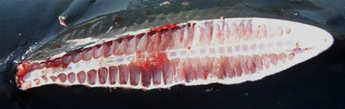
Figure 25: Cartilage from the fin of the Mako shark.
Source: © www.OrangeBeach.ws.
The shark has evolved very little in the last 400 million years and bears remarkable similarity to fossils of cartilaginous fish from the Devonian era, commonly known as the “Age of Fishes.” Presumably, the ancestors of today’s sharks were well-adapted to the warm inland seas blanketing the landscape at that time. In the present time, sharks seem to have reached an evolutionary dead end. They are well enough adapted to their environment and their genetic material is more or less static. As this photograph shows, they never developed a bony structure, and they also seem not to get cancer. (Unit: 9)
We can ask two questions based on what we have developed here: Is cancer an inevitable consequence of rapid evolution, and in that sense not a disease at all but a necessary outlier tail of rapid evolution? And is cancer, then, inevitably connected with high evolution rates and high stress conditions and thus impossible to “cure”?
Stress no doubt drives evolution forward, changing the fitness landscapes we have discussed from a basically smooth, flat, and boring plane into a rugged landscape of deep valleys and high peaks. Let us assume that in any local habitat or ecology is a distribution of genomes that includes some high-fitness genomes and some low-fitness genomes. The low-fitness genomes are under stress, but contain the seeds for evolution. We define stress here as something that either directly generates genomic damage, such as ionizing radiation and chemicals that directly attack DNA, viruses, or something that prevents replication of the genome, such as blockage of DNA polymerases or of the topological enzymes required for chromosome replication. Left unchallenged, all these stress inducers will result in the extinction of the quasi-species.
This is the business end of the grand experiment in exploring local fitness peaks and ultimately in generating resistance to stress. The system must evolve in response to the stress, and it must do this by deliberately generating genetic diversity to explore the fitness landscape—or not. Viewed in the perspective of game theory’s prisoner’s dilemma (see sidebar), the silent option under stress is not to evolve—to go down the senescent pathway and thus not attempt to propagate. Turning on mutational mechanisms, in contrast, is a defection, in the sense that it leads potentially to genomes which can propagate even in what should be lethal conditions and could, in principle, lead to the destruction of the organism: disease followed by death, which would seem to be very counterproductive. But it may well be a risk that the system is willing to make. If ignition of mutator genes and evolution to a new local maximum of fitness increases the average fitness of the group, then the inevitable loss of some individuals whose genome is mutated into a fitness valley is an acceptable cost.
7. Networks
The complex biological molecules we have spent the previous sections trying to understand are the building blocks of life, but it is far from obvious to put these building blocks together into a coherent whole. Biological molecules, as well as cells and complete organisms, are organized in complex networks. A network is defined as a system in which information flows into nodes, is processed, and then flows back out. The network’s output is a function of both the inputs and a series of edges that are the bidirectional paths of information flow between the nodes. The theory and practice of networks is a vast subject, and with one ultimate goal of understanding that greatest of mysteries, the human brain. We will return to the brain and its neural networks in the next section. For now, we will discuss the more prosaic networks in living organisms, which are still complex enough to be very intimidating.
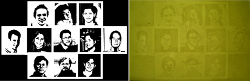
It isn’t obvious when you look at a cell that a network exists there. The cytoplasm of a living cell is a very dynamic entity, but at least at first glance seems to basically be a bag of biological molecules mixed chaotically together. It is somewhat of a shock to realize that this bag of molecules actually contains a huge number of highly specific biological networks all operating under tight control. For example, when an epithelial cell moving across a substrate, patterns of specific molecules drive the motion of the cell’s internal skeleton. When these molecules are tagged with a protein that glows red, displaying the collective molecular motion under a microscope, a very complex and interactive set of networks appears.

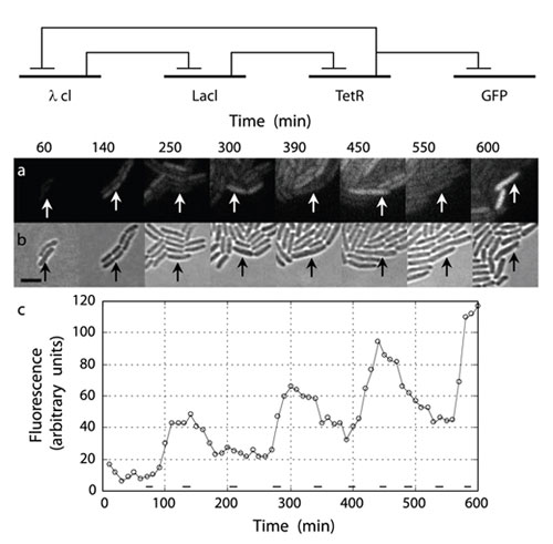
Figure 26: The circuit diagram (top), bacterial population (center), and plot of the dynamics (bottom) of the repressilator, an example of a simple synthetic biological network.
Source: © Top: Wikimedia Commons, Public Domain. Author: Timreid, 26 February 2007. Center and bottom: Reprinted by permission from Macmillan Publishers Ltd: Nature 403, 335-338 (20 January 2000).
The represillator is a simple synthetic biological network developed by Michael Elowitz and Stanislas Leibler. The network induces E. coli cells to periodically produce green fluorescent protein that can be observed under a microscope. It consists of three genes in a feedback loop, each of which represses the other genes, leading to oscillatory gene expression over time. The top image shows the equivalent circuit diagram for the repressilator. The center photographs show the total population of cells (bottom) compared to the green fluorescent portion of the population (top). The plot shows the total amount of green fluorescence over time: an oscillation superimposed on a general upward trend that matches population growth. (Unit: 9)
The emergent network of the cytoplasm is a system of interconnected units. Each unit has at least an input and an output, and some sort of a control input which can modulate the relationship between the input and the output. Networks can be analog, which means that in principle the inputs and outputs are continuous functions of some variable; or they can be digital, which means that they have finite values, typically 1 or 0 for a binary system. The computer on which this text was typed is a digital network consisting of binary logic gates, while the person who typed the text is an analog network.
There are many different kinds of biological networks, and they cover a huge range of length scales, from the submicron (a micron is a millionth of a meter) to the scales spanning the Earth. Outside of neural networks, the most important ones are (roughly in order of increasing abstraction):
- Metabolite networks: These networks control how a cell turns food (in the form of sugar) into energy that it can use to function. Enzymes (proteins) are the nodes, and the smaller molecules that represent the flow of chemical energy in the cell are the edges.
- Signal transduction networks: These networks transfer information from outside the cell into its interior, and translate that information into a set of instructions for activity within the cell. Proteins are the nodes, typically proteins called kineases, and diffusible small signaling molecules which have been chemically modified are the edges. This is a huge class of networks, ranging from networks that process sensory stimuli to chemical inputs such as hormones.
- Transcriptional regulatory networks: These networks determine how genes are turned on and off (or modulated).
- Interorganism networks: This is a very broad term that encompasses everything from the coordinated behavior of a group of bacteria to complex ecologies. The nodes are individual cells, and the edges are the many different physical ways that cells can interact with each other.
There are probably fundamental network design principles that must be obeyed independent of their biological or manmade (which is still biological) origin if the network is to be stable to perturbations. Instability in a network is not generally viewed as a good thing, although there are exceptions to this rule. For example, the aerodynamics of most modern fighter jets makes the plane inherently unstable. This sounds like a very bad thing, except that it makes the fighter extremely adaptive to direction changes. Modern computers can constantly monitor and instantaneously correct the instability, so we end up with aircraft that are far more maneuverable—and thus more effective fighters—than the ordinary, stable variety.
The kind of stability issues the fighter jet and other similar networks face are deterministic, and can be modeled by ordinary differential equations that are straightforward to write down. One might then imagine designing a network based on a set of these equations. One of the pioneering exercises in designing “from scratch” was the work of Elowitz and Leibler of an oscillating gene expression pattern. It is sobering to understand the depth of understanding that was necessary to have made this simple oscillator work. For an electrical engineer, it is straightforward to design an oscillator following some basic rules of electromagnetism. However, in a biological network, the parameters are much less cleanly defined. Despite the inherent challenges, we now have a basic set of biological modules that is being developed in the new field of “synthetic biology,” which is a mix of physics, engineering, and biology that exploits our knowledge of networks to design new functional biological “circuits.” Figure 27 shows an example of a biological “film” consisting of bacteria. To do this, a gene was inserted into E. coli that coded for a protein that causes the bacteria to make a black pigment. The pigment production was coupled to a light sensor, so that pigment would be made only in the dark. The group used stencils to pattern light exposure and produce bacterial photography.

Figure 27: Portrait of the University of Texas at Austin (UT Austin)/University of California, San Francisco (UCSF) Synthetic Biology team. The left panel shows the projected image of the students and professors from UT Austin and UCSF who participated in the project, and the right panel shows the resulting bacterial photo.
Source: © Aaron Chevalier and the University of Texas at Austin.
The photograph on the left shows members of the synthetic biology team at the University of Texas at Austin and the University of California, San Francisco. The team synthesized genetic material that coded for a black pigment and a light sensor, and inserted the gene into E. coli cells. The cells producing this protein turn black when kept in the dark, allowing the group to make photographic film out of a sheet of these bacteria. The image on the right shows the team members as captured by the bacteria they produced. (Unit: 9)
In addition to deterministic stability issues in biological networks, there is also the issue of stability in the presence of noise. For example, at the macro-scale, the sensory network of the dog’s nose is about a million times more sensitive than a human noise. Despite this extreme sensitivity, the dog nose is not overwhelmed by the presence of an enormous background of other molecules. That is, the dog nose sensory network is extremely good at noise rejection. At the micro-scale of the single cell, the very finite number of molecules actually involved in the network node edges leads to statistical noise that can either confound the network’s stability or increase its sensitivity. The dog has clearly resolved this issue to its benefit, but it remains a problem in the design of synthetic biological networks.
The obvious end goal of synthetic biology could be something truly astonishing: synthetic life. The key to synthetic life, if it is indeed achieved, will be our ability to harness biological networks. So far, scientists have synthesized genetic material and other important biological molecules from scratch, but have not put the pieces together into a complete living organism. The feat hailed by the media as the so-called creation of a “new form of life” by Craig Venter is something of a misnomer. While Venter’s synthesis of a functional bacterial chromosome of one million base pairs was a fantastic technical achievement, it is very far from synthetic life, as the new chromosome was inserted into an already functioning cell consisting of a enormous collection of interacting networks, which we neither can understand nor can reproduce. Until we can understand the emergence of life from the networks of biology, we will remain very far from achieving synthetic life.
8. The Emergence of the Mind
So far, we have wrestled with the structural diversity of proteins and its relationship to the free energy landscape, and we have tried to find some of the unifying and emergent properties of evolution that might explain the diversity of life and the increase in complexity. We have also taken a look at how the biological networks necessary to bind a collection of inanimate objects into a living system emerge. At the highest level lies the greatest mystery of biological physics: the emergence of the mind from a collection of communicating cells.

Figure 28: Ruby-throated hummingbird.
Source: © Steve Maslowski, U.S. Fish and Wildlife Service.
Hummingbirds, like the one pictured here, exemplify several areas of biological physics at once. Their mechanical properties are remarkable, especially their wings, with a high beat rate and large range of motion lending themselves to flight of which most airplane pilots can only dream. Their mental acuity is also impressive. Hummingbirds remember each flower they visit and calculate when the nectar supply is likely to be replenished, and need neither maps nor GPS to navigate accurately over thousands of miles. If we assume that the brain can be modeled as a computing machine, it’s an open question how a pea-sized computer can accomplish so much. (Unit: 9)
We started our discussion of biological physics by considering a chicken egg. Birds lay eggs, so let’s consider a bird: the ruby-throated hummingbird presented in all its glory in Figure 28. About 7 cm long and weighing about 5 grams, this bird is capable of some rather amazing biophysical things. Its wings beat about 50 times each second, and they rotate around their central axis through almost 180 degrees, allowing the bird to fly backwards and forwards and hover. A lot of these fascinating mechanical properties can be considered the subject of biological physics.
But there is far more to these hummingbirds than just flying ability. They live for about nine years, spend their summers in the northern parts of North America and their winters in tropical Central America. So, this small animal can navigate in the fall over thousands of miles, including over hundreds of miles of open water, to certain locations and then return in the spring to the region it was born. How is it that a tiny hummingbird can do all this remarkable navigation? The advancement in capabilities of the digital computer over the past 30 years has been truly staggering, yet it pales against what the hummingbird’s brain can do. The human brain is far more impressive. Why can a couple of pounds of neurons drawing a few watts of chemical power with an apparent clock speed of maybe a kilohertz at best do certain tasks far better than a machine the size of a large truck running megawatts of power? And at a much more troubling level, why do we speak of the soul of a person when no one at this point would seriously ascribe any sense of self-recognition to one of our biggest computers? We seem to be missing something very fundamental.
Traditional computers vs. biology
We have moved into the computer age via the pathway pioneered by British mathematician Alan Turing, whom we first met in the introduction to this unit. Our modern-day computers all basically use the model described in Figure 29, coupled with the idea that any number is to be presented by bits in a binary representation. We have made things much faster than those early computers, but the basic idea has not changed. Even the quantum computers promised in Unit 7 keep the same basic design, replacing binary bits with more powerful qubits.

Phineas Gage’s brain injury. © Wikimedia Commons, Public Domain.

Figure 29: Schematic of a modern digital computer.
A computer accepts an input and processes it by passing it through a logic unit (microprocessor), using random access memory for temporary information storage. A control unit coordinates information flow between the logic unit and memory. Finally, the processed information is output to the user. (Unit: 9)
But this is not how biology has developed its own computers. The basic design has four major flaws as far as biology is concerned:
- The machine must be told in advance, in great error-free detail, the steps needed to perform the algorithm.
- Data must be clean; the potential loss of a single bit can crash the code.
- The hardware must be protected and robust; one broken lead and the machine can crash.
- There is an exact correspondence between a bit of data and a hardware location: The information in the machine is localized.
None of this is any good for a biological system. As far as biology is concerned, our computers are evolutionary dead-ends. We started this unit by considering the fragility of the egg in a large fall. Yet, as the example of Phineas Gage in the side bar shows, our brain can take enormous abuse and remain basically functional. I challenged you initially to drop the possibly cooked egg and see what happens. Now I challenge you to take a 2 cm diameter steel rod and thrust it through your laptop with great force, then try to surf the web.
The brain of a nematode
The human brain is probably the most complex structure in the universe that we know, but not only humans have brains. The adult hermaphrodite of the “lowly” nematode C. elegans consists of only 959 cells; yet when you watch it navigating around on an agar plate, it certainly seems to be computing something based on its sensory input. The creature displays an astonishingly wide range of behavior: locomotion, foraging, feeding, defecation, egg laying, larva formation, and sensory responses to touch, smell, taste, and temperature, as well as some complex behaviors like mating, social behavior, and learning and memory. It would be quite hard to build a digital computer that could do all that, and certainly impossible to pack it into a tube about 1 mm long and a 100 microns in diameter that can reproduce itself.
The C. elegans doesn’t have a brain per se, but it does have about 302 information-carrying neurons that form approximately 7,000 synapses. We believe that any real brain capable of making some sort of a computation, as opposed to the collective behavior seen in single-celled organisms, must consist of neurons that transfer information. That information is not transferred to some sort of a central processing unit. Biological computers are systems of interconnected cells that transfer and process information. The network of neurons in C. elegans displays the common feature in interconnectivity: the synaptic connections formed by the neurons.
The brain versus the computer
I want to concentrate on one thing here: how differently the brain, even the pseudo-brain of C. elegans, is “wired” from the computer that you’re using to read this web page. Your computer has well-defined regions where critical functions take place: a section of random access memory (RAM) and a central processing unit (CPU). Each part is quite distinct, and buses transfer binary data between the different sections. Take out a single bus line or damage one of the RAM chips, and the system shuts down.
Brains in biology seem to have evolved in a different way. First, they are spatially diffuse. The computer is basically a two-dimensional device. Brains at every level seem to be basically three-dimensional. The interconnection takes place not via a bus, but rather through a vast network of input-output synaptic connections. For example, C. elegans has roughly 20 interconnects per neuron. In the human brain, we believe that the number is on the order of 103. Since the human brain has around 1012 neurons, the number of interconnects is on the order of 1015—a huge number.

Figure 30: Rainbow images showing individual neurons fluorescing in different colors. By tracking the neurons through stacks of slices, we can follow each neuron’s complex branching structure to create the treelike structures in the image on the right.
Source: © Jeff Lichtman, Center for Brain Science, Harvard University.
A research team at Harvard University has developed mice with brains that light up in a rainbow of colors. They developed a DNA sequence that codes for colorful fluorescent proteins, and inserted it into the mouse’s genome in a way that causes the color of each nerve cell to be selected at random. The image on the left shows the intricate structure of the mouse’s cerebellum. In the center, we see a portion of the brain’s cortex. In the brainbow images, it is possible to trace the path of each neuron through its complex branching structure to create treelike images like the one on the right. (Unit: 9)
It would be a mistake to think that the 1012 neurons in the brain correspond to about 1012 bits of information, or about 100 Gigabytes. The number is much higher, because of the three-dimensional interconnections linking each neuron with about 103 other neurons. Returning to our theme of spin glasses, we can estimate the information capacity by making the simple assumption that each neuron can be like a spin which is either up or down depending on its storage of a bit of information. This means that the total number of differing configurations of the brain is on the order of 21015, an absurdly huge number, far greater than even the number of atoms in the universe. We can only assume that the brains of living organisms emerged as they exploited this immense 3-D information capacity owing to the ability of communities of cells to form neuronal interconnections throughout space.
How does the brain reason?
Given the large information capacity of even a small network of neurons and the fact that the human brain’s capacity exceeds our ability to comprehend it, the next question is: How does a brain reason? As usual, we need to start by defining what we’re talking about. According to the Oxford English Dictionary, “reasoning” is “find[ing] a solution to a problem by considering possible options.” I suppose this dodges the question of the emergent property of consciousness, but I don’t see this problem being solved any time soon, although I hope I am wrong.
The hummingbird has a big problem, essentially asking itself: How shall I fly back to a place I was at six months ago that is thousands of miles away from where I am now? Presumably, the bird uses different physics than that of a traditional computer, because the information content that the bird has to sort out would cause it to fail catastrophically. So, we finally have the problem that perhaps physics can attack and clarify in the 21st century: How can a set of interacting neurons with a deep level of interconnects take previously stored information and determine an optimal solution to a problem it has not yet seen?
The hummingbird faces a problem rather reminiscent of the traveling salesman problem, explained in the sidebar. To choose the correct locations to pass through on its springtime journey north, it must consider a number of combinations far beyond the power of any computer system to resolve. How does the hummingbird do it? Is it magic?
Physics shows that it isn’t magic. As we have previously discussed, while a protein may fold or a species play with its genome in an almost uncountable number of ways, basic free energy minima schemes lead quite efficiently to a vastly smaller set of combinations that are roughly optimal. Nature doesn’t necessarily find the “best” solution, but it seems able to efficiently find a subset of solutions that works well enough. In the case of the traveling salesman problem, the vast combinatorics interconnects of a neural network of many neurons provides exactly the kind of search over a free energy surface that we need.
The “reasoning” ability of neural networks
We have discussed how landscapes—either fitness landscapes or free energy landscapes—can give rise to vastly complex surfaces with local minima representing some particular desired state. John Hopfield, a theoretical physicist at Princeton University, has explored ways for a system to find these minima. The three basic ideas below highlight how biological computers differ from their electronic counterparts:
- Neural networks are highly interconnected. This interaction network can be characterized by a matrix, which tabulates the interaction between each pair of neurons.
- Neurons interact in a nonlinear analog way. That is, the interconnection interaction is not an “all or nothing” matter, but a graded interaction where the firing rate of neurons varies smoothly with the input potential.
- An “energy function” can be constructed that allows us to understand the collective (or emergent) dynamics of the neuron network as it moves over the information landscapes and finds local minima that represent effective solutions to the problem.

Figure 31: An optimal traveling salesman problem (TSP) tour through Germany’s 15 largest cities. It is the shortest among 43,589,145,600 possible tours visiting each city exactly once.
Source: © Wikipedia, Creative Commons Attribution-ShareAlike License.
The traveling salesman problem, originally called the “Knight’s tour problem” by Euler, is a classic example of a simple optimization problem that is extremely difficult to solve in a reasonable amount of time. The blue line on this map of Germany shows the optimal path for a traveling salesman touring the fifteen most populous cities. This seemingly simple solution is one of over 43 billion possible routes. (Unit: 9)
Hopfield and molecular biologist David Tank set out to make an analogy between neural networks and the energy network of a glassy system characterized by a large number of degrees of freedom. Following the three principles outlined above, they used this analogy to write an equation for the free energy of a neural network in terms of the interaction between each pair of neurons, the threshold for each neuron to self-fire, and the potential for each of the neurons in the network. They also recognized that the interaction between pairs of neurons can change with time as the neural network learns.
The solution to a problem such as the traveling salesman problem emerges in the neural network as interaction strengths between the neutrons are adjusted to minimize the free energy equation. The flow of the neuron states during the computation can be mapped onto a flow on a free energy surface, similar to the flow of a spin glass toward its ground state or natural selection on a fitness landscape (but in the opposite direction). Clearly, quite complex and emergent neuronal dynamics can evolve with even the simple system we are considering here.
Hopfield and Tank showed that this neuronal map has quite impressive “reasoning” ability. A set of 900 neurons encoded to solve a 30-city traveling salesman problem was able to find 107 “best” solutions out of the 1030possible solutions, a rejection ratio of 1023 in just a few clock cycles of the neural network.
Although we clearly are a long way from understanding the emergent nature of consciousness, this example reveals the immense computational power of neural networks. Surely, one of the grand challenges in 21st century physics will be to move from these simple physical models derived from very concrete physics concepts to the vastly more complex terrain of the human brain.
9. Further Reading
- Howard Berg, movies of bacterial motion: http://webmac.rowland.org/labs/bacteria/index_movies.html.
- Michael B. Elowitz and Stanislas Leibler, “A Synthetic Oscillatory Network of Transcriptional Regulators,” Nature, 2000 Jan. 20; 403(6767): 335-8.
- Robert Laughlin, “A Different Universe: Reinventing Physics from the Bottom Down,” Basic Books, 2006.
- The National Human Genome Research Institute: http://www.genome.gov.