The Quantum World Online Textbook

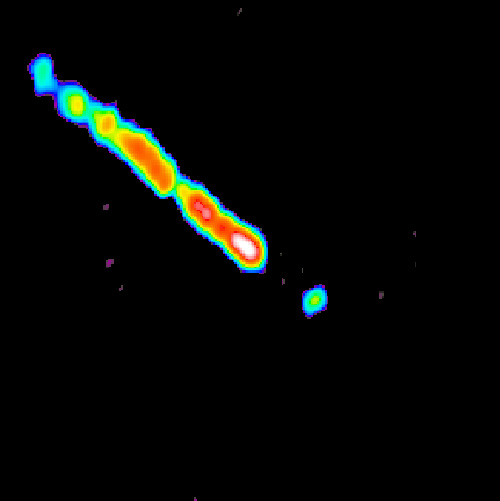
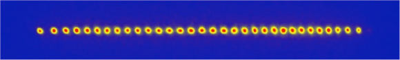
Figure 1: Thirty-two ions, fluorescing under illumination by laser light in an electrodynamic trap.
Source: © R. Blatt at Institut f. Experimentalphysik, Universtaet Innsbruck, Austria.
The observation of a single ion, held by an electrodynamic trap and fluorescing under laser light, marked the beginning of a new era in experimental quantum physics. Such an ion is at the heart of a new generation of atomic clocks. Here, we see a chain of ions in a linear trap. The chain can vibrate as a whole, and individual ions can be interrogated by laser light. This technology has helped to stimulate wide interest in quantum computing and quantum information science. (Unit: 5)

 

The creation of quantum mechanics in the 1920s broke open the gates to understanding atoms, molecules, and the structure of materials. This new knowledge transformed our world. Within two decades, quantum mechanics led to the invention of the transistor to be followed by the invention of the laser, revolutionary advances in semiconductor electronics, integrated circuits, medical diagnostics, and optical communications. Quantum mechanics also transformed physics because it profoundly changed our understanding of how to ask questions of nature and how to interpret the answers. An intellectual change of this magnitude does not come easily. The founders of quantum mechanics struggled with its concepts and passionately debated them. We are the beneficiaries of that struggle and quantum mechanics has now been developed into an elegant and coherent discipline. Nevertheless, quantum mechanics always seems strange on first acquaintance and certain aspects of it continue to generate debate today. We hope that this unit provides insight into how quantum mechanics works and why people find it so strange at first. We will also sketch some of the recent developments that have enormously enhanced our powers for working in the quantum world. These advances make it possible to manipulate and study quantum systems with a clarity previously achieved only in hypothetical thought experiments. They are so dramatic that some physicists have described them as a second quantum revolution.

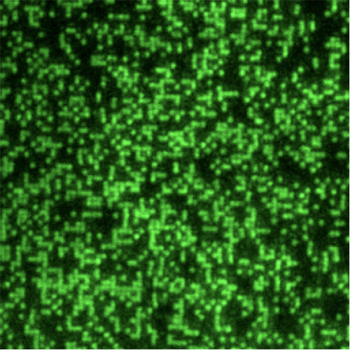
Figure 2: Neutral rubidium atoms in an optical lattice trap.
Source: © M. Greiner.
Ultracold atoms move so slowly that they can be confined by the weak force of light. Here, rubidium atoms are confined in an optical lattice made of standing light waves. The lattice, which is not visible in the image, creates a rectangular array of potential energy “buckets” in which individual atoms can be trapped. The lattice sites are separated by 640 nanometers. The lattice is a few layers deep and its rectangular structure is clearly visible. This system provides a new tool for studying theories of phenomena ranging from superconductivity to black holes. It also has potential applications for studies of quantum entanglement, quantum communication, and possibly quantum computing. (Unit: 5)

An early step in the second quantum revolution was the discovery of how to capture and manipulate a single ion in an electromagnetic trap, reduce its energy to the quantum limit, and even watch the ion by eye as it fluoresces. Figure 1 shows an array of fluorescing ions in a trap. Then methods were discovered for cooling atoms to microkelvin temperatures (a microkelvin is a millionth of a degree) and trapping them in magnetic fields or with light waves (Figure 2). These advances opened the way to stunning advances such as the observation of Bose-Einstein condensation of atoms, to be discussed in Unit 6, and the creation of a new discipline that straddles atomic and condensed matter physics.

The goal of this unit is to convey the spirit of life in the quantum world—that is, to give an idea of what quantum mechanics is and how it works—and to describe two events in the second quantum revolution: atom cooling and atomic clocks.

Figure 3: This furnace for melting glass is nearly an ideal blackbody radiation source.
Source: © OHM Equipment, LLC.
The outside of this glassblowing oven is clearly discernible, as is the front surface which is slightly darker than the interior. The crucible, which is almost at the oven temperature, is more difficult to discern. Except for the cool glassblower’s pipe, no features are visible within the oven because everything is at the same temperature and emits radiation identically. This oven provides a reasonable approximation of a blackbody. An even better approximation would be to seal the front of the oven, leaving only a small hole, so that the entire interior would be at exactly the same temperature. Any external light incident on the hole would be absorbed, and the only light radiated would come from the walls. Just such a technology was used for the early measurements on which Planck based his radiation law. (Unit: 5)

The nature of light was a profound mystery from the earliest stirrings of science until the 1860s and 1870s, when James Clerk Maxwell developed and published his electromagnetic theory. By joining the two seemingly disparate phenomena, electricity and magnetism, into the single concept of an electromagnetic field, Maxwell’s theory showed that waves in the field travel at the speed of light and are, in fact, light itself. Today, most physicists regard Maxwell’s theory as among the most important and beautiful theories in all of physics.

Maxwell’s theory is elegant because it can be expressed by a short set of equations. It is powerful because it leads to powerful predictions—for instance, the existence of radio waves and, for that matter, the entire electromagnetic spectrum from radio waves to x-rays. Furthermore, the theory explained how light can be created and absorbed, and provided a key to essentially every question in optics.

Given the beauty, elegance, and success of Maxwell’s theory of light, it is ironic that the quantum age, in which many of the most cherished concepts of physics had to be recast, was actually triggered by a problem involving light.

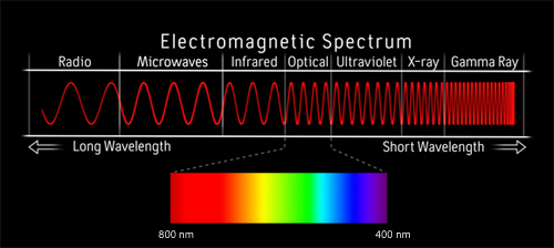
Figure 4: The electromagnetic spectrum from radio waves to gamma rays.
Maxwell’s Theory predicts the existence of electromagnetic radiation at essentially any wavelength or frequency. For obvious reasons, the mysteries of light were first explored in the optical region to which our eyes respond, but this represents only a minute fraction of the spectral regions that have been opened over the years. Electronic oscillators can generate electromagnetic waves with very long wavelengths. Lasers, hot filaments, light-emitting diodes (LEDs), and many other sources can generate light in the optical regime. X-rays are generated by electron collisions at medium energies, and the shortest wavelengths, ; (gamma) rays, are generated by high-energy nuclear collisions and in radioactive decay. The wave shown here in red is not to scale: The frequency of electromagnetic waves changes by over twenty orders of magnitude from the radio portion of the spectrum to gamma rays. (Unit: 5)

The spectrum of light from a blackbody—for instance the oven in Figure 3 or the filament of an electric light bulb—contains a broad spread of wavelengths. The spectrum varies rapidly with the temperature of the body. As the filament is heated, the faint red glow of a warm metal becomes brighter, and the peak of the spectrum broadens and shifts to a shorter wavelength, from orange to yellow and then to blue. The spectra of radiation from black bodies at different temperatures have identical shapes and differ only in the scales of the axes.

Figure 5: Spectrum of the cosmic microwave background radiation.
Source: © NASA, COBE.
The cosmic microwave background, which is thermal radiation left over from roughly 390,000 years after the Big Bang, has a nearly perfect blackbody spectrum. The shape of the curve and location of the peak indicate that the blackbody temperature of the CMB is 2.725 K. The shape of this universal curve of the blackbody spectrum posed a profound dilemma for theoretical physics. To explain the shape, Max Planck introduced his quantum hypothesis. Because he could not motivate his hypothesis, he found it difficult to believe his own theory. He used data taken by some colleagues who achieved incredible experimental expertise. The data shown here, taken by a satellite-borne radiometer called COBE, is so accurate that the error bars of the individual points all lie within the width of the plotted curve. (Unit: 5)

Enter the quantum

In the final years of the 19th century, physicists attempted to understand the spectrum of blackbody radiation but theory kept giving absurd results. German physicist Max Planck finally succeeded in calculating the spectrum in December 1900. However, he had to make what he could regard only as a preposterous hypothesis. According to Maxwell’s theory, radiation from a blackbody is emitted and absorbed by charged particles moving in the walls of the body, for instance by electrons in a metal. Planck modeled the electrons as charged particles held by fictitious springs. A particle moving under a spring force behaves like a harmonic oscillator. Planck found he could calculate the observed spectrum if he hypothesized that the energy of each harmonic oscillator could change only by discrete steps. If the frequency of the oscillator is ( is the Greek letter “nu” and is often used to stand for frequency), then the energy had to be 0, 1 hν, 2hν, 3 hν, … nhν, … where n could be any integer and h is a constant that soon became known as Planck’s constant. Planck named the stephν a quantum of energy. The blackbody spectrum Planck obtained by invoking his quantum hypothesis agreed beautifully with the experiment. But the quantum hypothesis seemed so absurd to Planck that he hesitated to talk about it.

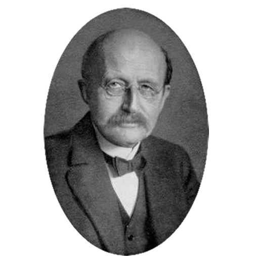
Figure 6: Max Planck solved the blackbody problem by introducing quanta of energy.
Source: © The Clendening History of Medicine Library, University of Kansas Medical Center
German physicist Max Planck (1848-1957) is widely regarded as one of the founders of quantum mechanics. He received the 1918 Nobel Prize in Physics for the work he began in an effort to calculate the spectrum of a blackbody from first principles. His seemingly preposterous postulate that energy of a harmonic oscillator could only change in discrete steps called quanta turned out to be a key concept in the new theory of quantum mechanics. (Unit: 5)

The physical dimension—the unit—of Planck’s constant h is interesting. It is either [energy] / [frequency] or [angular momentum]. Both of these dimensions have important physical interpretations. The constant’s value in S.I. units, 6.6 x 10^-34 joule-seconds, suggests the enormous distance between the quantum world and everyday events.

Planck’s constant is ubiquitous in quantum physics. The combination h/2 appears so often that it has been given a special symbol called “hbar.” This symbol appears in the upper-right-hand corner of these pages.

For five years, the quantum hypothesis had little impact. But in 1905, in what came to be called his miracle year, Swiss physicist Albert Einstein published a theory that proposed a quantum hypothesis from a totally different point of view. Einstein pointed out that, although Maxwell’s theory was wonderfully successful in explaining the known phenomena of light, these phenomena involved light waves interacting with large bodies. Nobody knew how light behaved on the microscopic scale—with individual electrons or atoms, for instance. Then, by a subtle analysis based on the analogy of certain properties of blackbody radiation with the behavior of a gas of particles, he concluded that electromagnetic energy itself must be quantized in units of . Thus, the light energy in a radiation field obeyed the same quantum law that Planck proposed for his fictitious mechanical oscillators; but Einstein’s quantum hypothesis did not involve hypothetical oscillators.

An experimental test of the quantum hypothesis

Whereas Planck’s theory led to no experimental predictions, Einstein’s theory did. When light hits a metal, electrons can be ejected, a phenomenon called the photoelectric effect. According to Einstein’s hypothesis, the energy absorbed by each electron had to come in bundles of light quanta. The minimum energy an electron could extract from the light beam is one quantum, hν. A certain amount of energy, W, is needed to remove electrons from a metal; otherwise they would simply flow out. So, Einstein predicted that the maximum kinetic energy of a photoelectron, E, had to be given by the equation E=hν – W.

The prediction is certainly counterintuitive, for Einstein predicted that E would depend only on the frequency of light, not on the light’s intensity. The American physicist Robert A. Millikan set out to prove experimentally that Einstein must be wrong. By a series of painstaking experiments, however, Millikan convinced himself that Einstein must be right.

The quantum of light energy is called a photon. A photon possesses energy hν, and it carries momentum hν/c, where c is the speed of light. Photons are particle-like because they carry discrete energy and momentum. They are relativistic because they always travel at the speed of light and consequently can possess momentum even though they are massless.

Although the quantum hypothesis solved the problem of blackbody radiation, Einstein’s concept of a light quantum—a particle-like bundle of energy—ran counter to common sense because it raised a profoundly troubling question: Does light consist of waves or particles? As we will show, answering this question required a revolution in physics. The issue was so profound that we should devote the next section to reviewing just what we mean by a wave and what we mean by a particle.

A particle is an object so small that its size is negligible; a wave is a periodic disturbance in a medium. These two concepts are so different that one can scarcely believe that they could be confused. In quantum physics, however, they turn out to be deeply intertwined and fundamentally inseparable.

Figure 7: A circular wave created by tossing a pebble in a pond.
Source: © Adam Kleppner.
There is no better way to study waves than by tossing pebbles into a pond on a calm sunny day. A single pebble causes a spreading circular wave, as shown here. This wave only continues for a few wavelengths, but if the disturbance were periodic, a steady stream of waves would be generated. Clearly, the energy of the splash is being carried outward in all directions. Tossing a couple of pebbles nearby creates a set of circular waves that magically pass through each other, demonstrating the principle of superposition that plays an almost magical role in quantum mechanics. If the wave amplitude becomes very high, the waves interact with each other and there is a breakdown of superposition. (Unit: 5)

The electron provides an ideal example of a particle because no attempt to measure its size has yielded a value different from zero. Clearly, an electron is small compared to an atom, while an atom is small compared to, for instance, a marble. In the night sky, the tiny points of starlight appear to come from luminous particles, and for many purposes we can treat stars as particles that interact gravitationally. It is evident that “small” is a relative term. Nevertheless, the concept of a particle is generally clear.

The essential properties of a particle are its mass, m; and, if it is moving with velocity v, its momentum, mv; and its kinetic energy, 1/2mv ². The energy of a particle remains localized, like the energy of a bullet, until it hits something. One could say, without exaggeration, that nothing could be simpler than a particle.

Figure 8: Two waves interfere as they cross paths.
Source: © Eli Sidman, Technical Services Group, MIT.
This photograph of a ripple tank shows the interference of two water waves. The waves are excited by two vibrating probes near the top of the photograph. Blue circles have been added at the wave crests. Where the circles cross, the amplitudes add to produce a large displacement. In between, the displacement of one wave is canceled by the opposite displacement of the other. (Unit: 5)

A wave is a periodic disturbance in a medium. Water waves are the most familiar example (we talk here about gentle waves, like ripples on a pond, not the breakers loved by surfers); but there are numerous other kinds, including sound waves (periodic oscillations of pressure in the air), light waves (periodic oscillations in the electromagnetic field), and the yet-to-be-detected gravitational waves (periodic oscillations in the gravitational field). The nature of the amplitude, or height of the wave, depends on the medium, for instance the pressure of air in a sound wave, the actual height in a water wave, or the electric field in a light wave. However, every wave is characterized by its wavelength (the Greek letter “lambda”), the distance from one crest to the next; its frequency (the Greek letter “nu”), the number of cycles or oscillations per second; and its velocity v, the distance a given crest moves in a second. This distance is the product of the number of oscillations the wave undergoes in a second and the wavelength.

Figure 9: Standing waves on a string between two fixed endpoints.
Source: © Daniel Kleppner.

The energy in a wave spreads like the ripples traveling outward in Figure 7. A surprising property of waves is that they pass freely through each other: as they cross, their displacements simply add. The wave fronts retain their circular shape as if the other wave were not there. However, at the intersections of the circles marking the wave crests, the amplitudes add, producing a bright image. In between, the positive displacement of one wave is canceled by the negative displacement of the other. This phenomenon, called interference, is a fundamental property of waves. Interference constitutes a characteristic signature of wave phenomena.

If a system is constrained, for instance if the medium is a guitar string that is fixed at either end, the energy cannot simply propagate away. As a result, the pattern is fixed in space and it oscillates in time. Such a wave is called a standing wave.

Far from their source, in three dimensions, the wave fronts of a disturbance behave like equally spaced planes, and the waves are called plane waves. If plane waves pass through a slit, the emerging wave does not form a perfect beam but spreads, or diffracts, as in Figure 10. This may seem contrary to experience because light is composed of waves, but light waves do not seem to spread. Rather, light appears to travel in straight lines. This is because in everyday experience, light beams are formed by apertures that are many wavelengths wide. A 1 millimeter aperture, for instance, is about 2,000 wavelengths wide. In such a situation, diffraction is weak and spreading is negligible. However, if the slit is about a wavelength across, the emerging disturbance is not a sharp beam but a rapidly spreading wave, as in Figure 10. To see light diffract, one must use very narrow slits.

Figure 11: Diffraction of laser light through one (top) and two (bottom) small slits.
Source: © Eli Sidman, Technical Services Group, MIT.
The upper trace shows a close to perfect single-slit diffraction pattern created by passing red laser light through a narrow slit. Most of the light is in the center lobe, but four additional lobes are clearly visible on either side. The lower trace displays the effect of combining diffraction patterns that are from slits close together. The bead-like appearance arises from the periodic two-slit interference pattern that is superimposed on the individual one-slit diffraction patterns. (Unit: 5)

If a plane wave passes through two nearby slits, the emerging beams can overlap and interfere. The points of interference depend only on the geometry and are fixed in space. The constructive interference creates a region of brightness, while destructive interference produces darkness. As a result, the photograph of light from two slits reveals bright and dark fringes, called “interference fringes.” An example of two-slit interference is shown in Figure 11.

The paradox emerges

Diffraction, interference, and in fact all of the phenomena of light can be explained by the wave theory of light, Maxwell’s theory. Consequently, there can be no doubt that light consists of waves. However, in Section 2 we described Einstein’s conjecture that light consists of particle-like bundles of energy, and explained that the photoelectric effect provides experimental evidence that this is true. A single phenomenon that displays contrary properties creates a paradox.

Is it possible to reconcile these two descriptions? One might argue that the bundles of light energy are so small that their discreteness is unimportant. For instance, a one-watt light source, which is quite dim, emits over 10¹⁸photons per second. The number of photons captured in visual images or the images in digital cameras are almost astronomically large. One photon more or less would never make a difference. However, we will see show examples where wave-like behavior is displayed by single particles. We will return to the wave-particle paradox later.

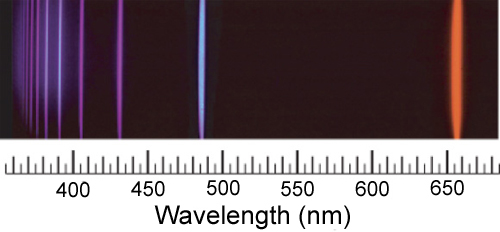
Early in the 20th century, it was known that everyday matter consists of atoms and that atoms contain positive and negative charges. Furthermore, each type of atom, that is, each element, has a unique spectrum—a pattern of wavelengths the atom radiates or absorbs if sufficiently heated. A particularly important spectrum, the spectrum of atomic hydrogen, is shown in Figure 12. The art of measuring the wavelengths, spectroscopy, had been highly developed, and scientists had generated enormous quantities of precise data on the wavelengths of light emitted or absorbed by atoms and molecules.

Figure 12: The spectrum of atomic hydrogen.
Source: © T.W. Hänsch.
This spectrum of atomic hydrogen was taken as an exercise by T. W Hänsch early in his career while he was pioneering laser spectroscopy. This group of spectral lines, known as the Balmer series, played a crucial role for Niels Bohr as he developed his model of the atom. Hänsch continued to refine hydrogen spectroscopy over the years and has obtained an absolute precision of a few parts in 1014. This research program also led to the invention of the optical frequency comb, which plays a critical role in the precise atomic clocks described in Section 8. (Unit: 5)

In spite of the elegance of spectroscopic measurement, it must have been uncomfortable for scientists to realize that they knew essentially nothing about the structure of atoms, much less why they radiate and absorb certain colors of light. Solving this puzzle ultimately led to the creation of quantum mechanics, but the task took about 20 years.

The nuclear atom

In 1910, there was a major step in unraveling the mystery of matter: Ernest Rutherford realized that most of the mass of an atom is located in a tiny volume—a nucleus—at the center of the atom. The positively charged nucleus is surrounded by the negatively charged electrons. Rutherford was forced reluctantly to accept a planetary model of the atom in which electrons, electrically attracted to the nucleus, fly around the nucleus like planets gravitationally attracted to a star. However, the planetary model gave rise to a dilemma. According to Maxwell’s theory of light, circling electrons radiate energy. The electrons would generate light at ever-higher frequencies as they spiraled inward to the nucleus. The spectrum would be broad, not sharp. More importantly, the atom would collapse as the electrons crashed into the nucleus. Rutherford’s discovery threatened to become a crisis for physics.

The Bohr model of hydrogen

Niels Bohr, a young scientist from Denmark, happened to be visiting Rutherford’s laboratory and became intrigued by the planetary atom dilemma. Shortly after returning home Bohr proposed a solution so radical that even he could barely believe it. However, the model gave such astonishingly accurate results that it could not be ignored. His 1913 paper on what became known as the “Bohr model” of the hydrogen atom opened the path to the creation of quantum mechanics.

Figure 13: Bohr’s model of an atom.
Source: © Daniel Kleppner.
Niels Bohr’s model of hydrogen depicts the atom as a small, positively charged nucleus surrounded by electrons that travel in circular orbits around the nucleus—similar in structure to the solar system, but with electrostatic forces providing attraction, rather than gravity. The Bohr model has become a logo for nuclear physics, with a few elliptical orbits artfully displayed. However, Bohr himself did not take it literally, and it has been totally superseded by quantum mechanics. Bohr’s model is essentially mechanistic with quantum ideas imposed on the allowed energies. In his model, elliptical as well as circular orbits are possible. (Unit: 5)

Bohr proposed that—contrary to all the rules of classical physics—hydrogen atoms exist only in certain fixed energy states, called stationary states. Occasionally, an atom somehow jumps from one state to another by radiating the energy difference. If an atom jumps from state b with energy E_b to state a with lower energy, E_a, it radiates light with frequency given by . Today, we would say that the atom emits a photon when it makes a quantum jump. The reverse is possible: An atom in a lower energy state can absorb a photon with the correct energy and make a transition to the higher state. Each energy state would be characterized by an integer, now called a quantum number, with the lowest energy state described by n = 1.

Bohr’s ideas were so revolutionary that they threatened to upset all of physics. However, the theories of physics, which we now call “classical physics,” were well tested and could not simply be dismissed. So, to connect his wild proposition with reality, Bohr introduced an idea that he later named the Correspondence Principle. This principle holds that there should be a smooth transition between the quantum and classical worlds. More precisely, in the limit of large energy state quantum numbers, atomic systems should display classical-like behavior. For example, the jump from a state with quantum number n = 100 to the state n = 99 should give rise to radiation at the frequency of an electron circling a proton with approximately the energy of those states. With these ideas, and using only the measured values of a few fundamental constants, Bohr calculated the spectrum of hydrogen and obtained astonishing agreement with observations.

Bohr understood very well that his theory contained too many radical assumptions to be intellectually satisfying. Furthermore, it left numerous questions unanswered, such as why atoms make quantum jumps. The fundamental success of Bohr’s model of hydrogen was to signal the need to replace classical physics with a totally new theory. The theory should be able to describe behavior at the microscopic scale—atomic behavior—but it should also be in harmony with classical physics, which works well in the world around us.

Matter waves

By the end of the 1920s, Bohr’s vision of a new theory was fulfilled by the creation of quantum mechanics, which turned out to be strange and even disturbing.

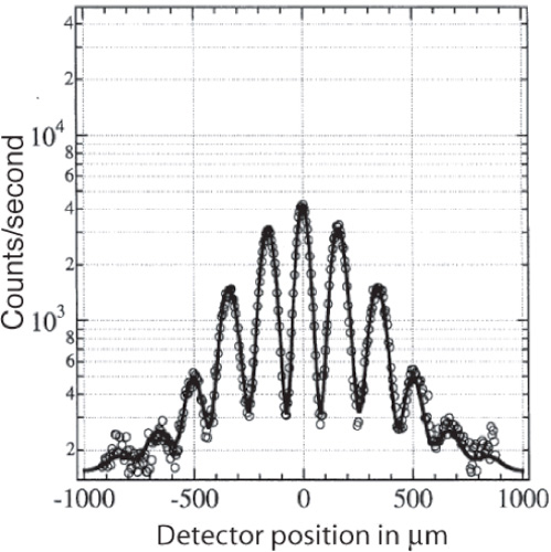
Figure 14: This diffraction pattern appeared when a beam of sodium molecules encountered a series of small slits, showing their wave-like nature.
Source: © D.E. Pritchard.
The diffraction pattern shown here was generated by placing a diffraction grating with a series of slits spaced 100 µm apart in the path of a beam of sodium molecules. Showing their wave-like nature, the molecules are diffracted from the slits similarly to the laser light in Figure 11. The circles on the plot show the number of molecules detected at different distances from the center of the beam. The solid line is a fit matching theory to the experimental data. (Unit: 5)

A key idea in the development of quantum mechanics came from the French physicist Louis de Broglie. In his doctoral thesis in 1924, de Broglie suggested that if waves can behave like particles, as Einstein had shown, then one might expect that particles can behave like waves. He proposed that a particle with momentum p should be associated with a wave of wavelength = h/p, where, as usual, h stands for Planck’s constant. The question “Waves of what?” was left unanswered.

de Broglie’s hypothesis was not limited to simple particles such as electrons. Any system with momentum p, for instance an atom, should behave like a wave with its particular de Broglie wavelength. The proposal must have seemed absurd because in the entire history of science, nobody had ever seen anything like a de Broglie wave. The reason that nobody had ever seen a de Broglie wave, however, is simple: Planck’s constant is so small that the de Broglie wavelength for observable everyday objects is much too small to be noticeable. But for an electron in hydrogen, for instance, the deBroglie wavelength is about the size of the atom.

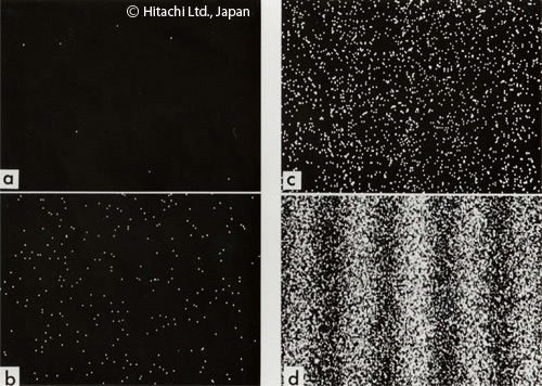
Figure 15: An interference pattern builds up as individual electrons pass through two slits.
Source: © Reprinted courtesy of Dr. Akira Tonomura, Hitachi, Ltd., Japan.
An interference pattern builds up on a sensitive detector as electrons pass through two slits, demonstrating both their wave and particle properties. In panel a, eight electrons appear to be randomly scattered on the detector after passing though the slits. As more electrons pass through the slits onto the detector, the pattern appears increasingly less random (panels b and c), until finally a two-slit interference pattern emerges in panel d, which shows the position of 60,000 electrons. The double slit in this experiment was formed in an electron microscope by sending a beam of high energy electrons on either side of a filament with a diameter less than a micrometer. The detector is sensitive enough to detect individual electrons with almost 100% efficiency. (Unit: 5)

Today, de Broglie waves are familiar in physics. For example, the diffraction of particles through a series of slits (see Figure 14) looks exactly like the interference pattern expected for a light wave through a series of slits. The signal, however, is that of a matter wave—the wave of a stream of sodium molecules. The calculated curve (solid line) is the interference pattern for a wave with the de Broglie wavelength of sodium molecules, which are diffracted by slits with the measured dimensions. The experimental points are the counts from an atom (or molecule) detector. The stream of particles behaves exactly like a wave.

The concept of a de Broglie wave raises troubling issues. For instance, for de Broglie waves one must ask: Waves of what? Part of the answer is provided in the two-slit interference data in Figure 15. The particles in this experiment are electrons. Because the detector is so sensitive, the position of every single electron can be recorded with high efficiency. Panel (a) displays only eight electrons, and they appear to be randomly scattered. The points in panels (b) and (c) also appear to be randomly scattered. Panel (d) displays 60,000 points, and these are far from randomly distributed. In fact, the image is a traditional two-slit interference pattern. This suggests that the probability that an electron arrives at a given position is proportional to the intensity of the interference pattern there. It turns out that this suggestion provides a useful interpretation of a quantum wavefunction: The probability of finding a particle at a given position is proportional to the intensity of its wavefunction there, that is to the square of the wavefunction.

As we saw in the previous section, there is strong evidence that atoms can behave like waves. So, we shall take the wave nature of atoms as a fact and turn to the questions of how matter waves behave and what they mean.

Figure 16: Werner Heisenberg (left) and Erwin Schrödinger (right).
Source: © Left: German Federal Archive, Creative Commons Attribution ShareAlike 3.0 Germany License. Right: Francis Simon, courtesy AIP Emilio Segrè Visual Archives.
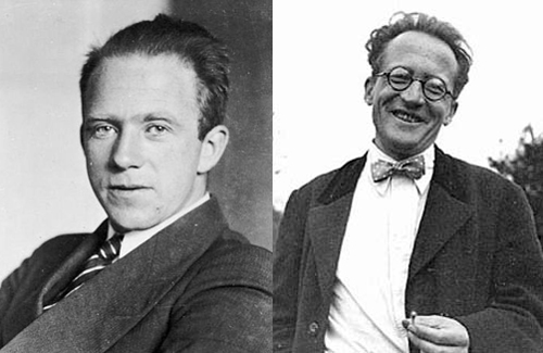
Werner Heisenberg (left) and Erwin Schrödinger (right) are two of the founding fathers of modern quantum mechanics. Schrödinger’s formulation of a wave equation for particles, and his various solutions to it, gave rigorous answers to seeming paradoxes of quantum mechanics. Heisenberg developed an alternate formulation of quantum mechanics in terms of what was considered new math at the time: matrices and linear algebra. (Unit: 5)

Mathematically, waves are described by solutions to a differential equation called the “wave equation.” In 1925, the Austrian physicist Erwin Schrödinger reasoned that since particles can behave like waves, there must be a wave equation for particles. He traveled to a quiet mountain lodge to discover the equation; and after a few weeks of thinking and skiing, he succeeded. Schrödinger’s equation opened the door to the quantum world, not only answering the many paradoxes that had arisen, but also providing a method for calculating the structure of atoms, molecules, and solids, and for understanding the structure of all matter. Schrödinger’s creation, called wave mechanics, precipitated a genuine revolution in science. Almost simultaneously, a totally different formulation of quantum theory was created by Werner Heisenberg: matrix mechanics. The two theories looked different but turned out to be fundamentally equivalent. Often, they are simply referred to as “quantum mechanics.” Schrödinger and Heisenberg were awarded the Nobel Prize in 1932 for their theories.

In wave mechanics, our knowledge about a system is embodied in its wavefunction. A wavefunction is the solution to Schrödinger’s equation that fits the particular circumstances. For instance, one can speak of the wavefunction for a particle moving freely in space, or an electron bound to a proton in a hydrogen atom, or a mass moving under the spring force of a harmonic oscillator.

To get some insight into the quantum description of nature, let’s consider a mass M, moving in one dimension, bouncing back and forth between two rigid walls separated by distance L. We will refer to this idealized one-dimensional system as a particle in a box. The wavefunction must vanish outside the box because the particle can never be found there. Physical waves cannot jump abruptly, so the wavefunction must smoothly approach zero at either end of the box. Consequently, the box must contain an integral number of half-wavelengths of the particle’s de Broglie wave. Thus, the de Broglie wavelength λ must obey nλ/2=L, where L is the length of the box and n = 1, 2, 3… . The integer n is called the quantum number of the state. Once we know the de Broglie wavelength, we also know the particle’s momentum and energy.  See The Math section below.

Figure 17: The first three allowed de Broglie wave modes for a particle in a box.
Source: © Daniel Kleppner.
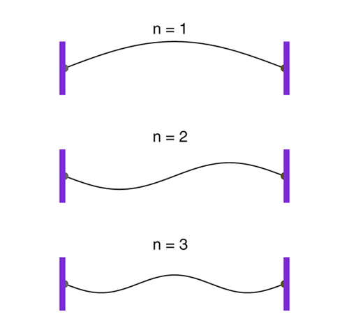
These wave modes, which correspond to the three lowest energy de Broglie waves of a particle moving in a one-dimensional box (defined by the purple bars), are identical to the patterns for the modes on a string in Figure 9. The waves on a string result from the physical displacement of the string from equilibrium. The physical meaning of de Broglie waves is yet to be discussed. Nevertheless, their existence immediately leads to the concept of energy quantization. In this case, the energy levels increase as n2. (Unit: 5)

The mere existence of matter waves suggests that in any confined system, the energy can have only certain discrete values, that is the energy is quantized. The minimum energy is called the ground state energy. For the particle in the box, the ground state energy is (hL)²/8M. The energy of the higher-lying states increases as n². For a harmonic oscillator, it turns out that the energy levels are equally spaced, and the allowed energies increase linearly with n. For a hydrogen atom, the energy levels are found to get closer and closer as n increases, varying as 1/n².

If this is your first encounter with quantum phenomena, you may be confused as to what the wavefunction means and what connection it could have with the behavior of a particle. Before discussing the interpretation, it will be helpful to look at the wavefunction for a system slightly more interesting than a particle in a box.

The harmonic oscillator

Figure 18: A simple harmonic oscillator (bottom) and its energy diagram (top).
Source: © Daniel Kleppner.

In free space, where there are no forces, the momentum and kinetic energy of a particle are constant. In most physically interesting situations, however, a particle experiences a force. A harmonic oscillator is a particle moving under the influence of a spring force as shown in Figure 18. The spring force is proportional to how far the spring is stretched or compressed away from its equilibrium position, and the particle’s potential energy is proportional to that distance squared. Because energy is conserved, the total energy, E = K + V, is constant. These relations are shown in the energy diagram in Figure 18.

The energy diagram in Figure 18 is helpful in understanding both classical and quantum behavior. Classically, the particle moves between the two extremes (-a, a) shown in the drawing. The extremes are called “turning points” because the direction of motion changes there. The particle comes to momentary rest at a turning point, the kinetic energy vanishes, and the potential energy is equal to the total energy. When the particle passes the origin, the potential energy vanishes, and the kinetic energy is equal to the total energy. Consequently, as the particle moves back and forth, its momentum oscillates between zero and its maximum value.

Figure 19: Low-lying energy levels of a harmonic oscillator.
Source: © Daniel Kleppner.

Solutions to Schrödinger’s equation for the harmonic oscillator show that the energy is quantized, as we expect for a confined system, and that the allowed states are given by E_n = (n+1/2)hν, where  is the frequency of the oscillator and n = 0, 1, 2… . The energy levels are separated by hν, as Planck had conjectured, but the system has a ground state energy 1/2hν, which Planck could not have known about. The harmonic oscillator energy levels are evenly spaced, as shown in Figure 19.

What does the wavefunction mean?

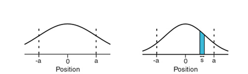
If we measure the position of the mass, for instance by taking a flash photograph of the oscillator with a meter stick in the background, we do not always get the same result. Even under ideal conditions, which includes eliminating thermal fluctuations by working at zero temperature, the mass would still jitter due to its zero point energy. However, if we plot the results of successive measurements, we find that they start to look reasonably orderly. In particular, the fraction of the measurements for which the mass is in some interval, s, is proportional to the area of the strip of width s lying under the curve in Figure 20, shown in blue. This curve is called a probability distribution curve. Since the probability of finding the mass somewhere is unity, the height of the curve must be chosen so that the area under the curve is 1. With this convention, the probability of finding the mass in the interval s is equal to the area of the shaded strip. It turns out that the probability distribution is simply the wavefunction squared.

Figure 20: The ground state wavefunction of a harmonic oscillator (left) and the corresponding probability distribution (right).
Source: © Daniel Kleppner

Here, we have a curious state of affairs. In classical physics, if one knows the state of a system, for instance the position and speed of a marble at rest, one can predict the result of future measurements as precisely as one wishes. In quantum mechanics, however, the harmonic oscillator cannot be truly at rest: The closest it can come is the ground state energy 1/2 . Furthermore, we cannot predict the precise result of measurements, only the probability that a measurement will give a result in a given range. Such a probabilistic theory was not easy to accept at first. In fact, Einstein never accepted it.

Aside from its probabilistic interpretation, Figure 20 portrays a situation that could hardly be less like what we expect from classical physics. A classical harmonic oscillator moves fastest near the origin and spends most of its time as it slows down near the turning points. Figure 20 suggests the contrary: The most likely place to find the mass is at the origin where it is moving fastest. However, there is an even more bizarre aspect to the quantum solution: The wavefunction extends beyond the turning points. This means that in a certain fraction of measurements, the mass will be found in a place where it could never go if it obeyed the classical laws. The penetration of the wavefunction into the classically forbidden region gives rise to a purely quantum phenomenon called tunneling. If the energy barrier is not too high, for instance if the energy barrier is a thin layer of insulator in a semiconductor device, then a particle can pass from one classically allowed region to another, tunneling through a region that is classically forbidden.

The quantum description of a harmonic oscillator starts to look a little more reasonable for higher-lying states. For instance, the wavefunction and probability distribution for the state n = 10 are shown in Figure 21.

Figure 21: The wavefunction (left) and probability distribution (right) of a harmonic oscillator in the state n = 10.
Source: © Daniel Kleppner.
The n = 40 wavefunction for the harmonic oscillator, found by solving Schrödinger’s equation, is shown on the left. The corresponding probability distribution, which oscillates rapidly in space, is shown on the right. As the quantum number n increases, the oscillation rate increases, and the probability of finding the particle in a given region approximates a smooth curve at the average height of each oscillation. In classical physics, the probability of finding the particle at a particular position is proportional to the fraction of time the particle spends there, which is inversely proportional to the particle’s velocity. The particle therefore is most likely to be found at a turning point, and spends much less time near the equilibrium position. The classical and the quantum predictions get closer and closer as n increases, with one important exception: The classical curve diverges at the turning point where the particle has zero velocity, while the quantum curve is smoothed over. This is a characteristic difference between the quantum and classical pictures. (Unit: 5)

Although the n = 10 state shown in Figure 21 may look weird, it shows some similarities to classical behavior. The mass is most likely to be observed near a turning point and least likely to be seen near the origin, as we expect. Furthermore, the fraction of time it spends outside of the turning points is much less than in the ground state. Aside from these clues, however, the quantum description appears to have no connection to the classical description of a mass oscillating in a real harmonic oscillator. We turn next to showing that such a connection actually exists.

The idea of the position of an object seems so obvious that the concept of position is generally taken for granted in classical physics. Knowing the position of a particle means knowing the values of its coordinates in some coordinate system. The precision of those values, in classical physics, is limited only by our skill in measuring. In quantum mechanics, the concept of position differs fundamentally from this classical meaning. A particle’s position is summarized by its wavefunction. To describe a particle at a given position in the language of quantum mechanics, we would need to find a wavefunction that is extremely high near that position and zero elsewhere. The wavefunction would resemble a very tall and very thin tower. None of the wavefunctions we have seen so far look remotely like that. Nevertheless, we can construct a wavefunction that approximates the classical description as precisely as we please.

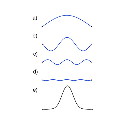
Let’s take the particle in a box described in Section 4 as an example. The possible wavefunctions, each labeled by an integer quantum number, n, obey the superposition principle, and so we are free to add solutions with different values of n, adjusting the amplitudes as needed. The sum of the individual wavefunctions yields another legitimate wavefunction that could describe a particle in a box. If we’re clever, we can come up with a combination that resembles the classical solution. If, for example, we add a series of waves with n = 1, 3, 5, and 7 and the carefully chosen amplitudes shown in Figure 22, the result appears to be somewhat localized near the center of the box.

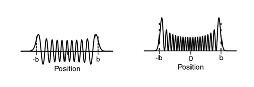
Figure 22: Some wavefunctions for a particle in a box. Curve (e) is the sum of curves (a-d).
Source: © Daniel Kleppner.
The blue lines (a-d) show the n = 1, 3, 5, and 7 wavefunctions for a particle in a one-dimensional box. The black line (e) is the sum of these wavefunctions, which itself is a solution of Schrödinger’s equation. It is remarkable that four wiggly curves add to give a smooth curve, but the computation is highly precise. As additional curves of shorter wavelengths are added, the resultant peak becomes narrower and narrower. Thus, in principle, the particle can be precisely localized. However, the spread in momentum would be enormous. (Unit: 5)

Localizing the particle has come at a cost, however, because each wave we add to the wavefunction corresponds to a different momentum. If the lowest possible momentum is p₀, then the wavefunction we created has components of momentum at p₀, 3p₀, 5p₀, and 7p₀. If we measure the momentum, for instance, by suddenly opening the ends of the box and measuring the time for the particle to reach a detector, we would observe one of the four possible values. If we repeat the measurement many times and plot the results, we would find that the probability for a particular value is proportional to the square of the amplitude of its component in the wavefunction.

If we continue to add waves of ever-shortening wavelengths to our solution, the probability curve becomes narrower while the spread of momentum increases. Thus, as the wavefunction sharpens and our uncertainty about the particle’s position decreases, the spread of values observed in successive measurements, that is, the uncertainty in the particle’s momentum, increases.

This state of affairs may seem unnatural because energy is not conserved: Often, the particle is observed to move slowly but sometimes it is moving very fast. However, there is no reason energy should be conserved because the system must be freshly prepared before each measurement. The preparation process requires that the particle has the given wavefunction before each measurement. All the information that we have about the state of a particle is in its wavefunction, and this information does not include a precise value for the energy.

The reciprocal relation between the spread in repeated measurements of position and momentum was first recognized by Werner Heisenberg. If we denote the scatter in results for repeated measurements of a position of a particle byΔx (Δ, Greek letter “delta”), and the scatter in results in repeated measurements of the momentum byΔp, then Heisenberg showed that ΔxΔp ≥ h/4π, a result famously known as the Heisenberg uncertainty principle. The uncertainty principle means that in quantum mechanics, we cannot simultaneously know both the position and the momentum of an object arbitrarily well.

Measurements of certain other quantities in quantum mechanics are also governed by uncertainty relations. An important relation for quantum measurements relates the uncertainty in measurements of the energy of a system, ΔE, to the time τ (τ, Greek letter “tau”) during which the measurement is made: τΔE ≥h/4π .

Some illustrations of the uncertainty principle

Harmonic oscillator. The ground state energy of the harmonic oscillator, 1/2hv, makes immediate sense from the uncertainty principle. If the ground state of the oscillator were more highly localized, that is sharper than in Figure 20, the oscillator’s average potential energy would be lower. However, sharpening the wavefunction requires introducing shorter wavelength components. These have higher momentum, and thus higher kinetic energy. The result would be an increase in the total energy. The ground state represents the optimum trade-off between decreasing the potential energy and increasing the kinetic energy.

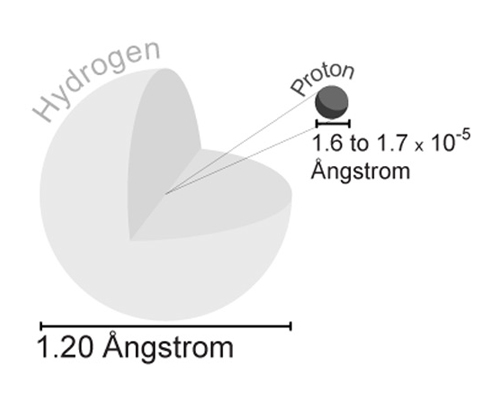
Figure 23: The size of a hydrogen atom is determined by the uncertainty principle.
Source: © Wikimedia Commons, Public Domain. Author: Bensaccount, 10 July 2006
A hydrogen atom is around one hundred thousand times larger than the proton that forms its nucleus. If we think of the electron as smeared over a spherical volume, this volume is enormous compared to the proton. This volume is the result of balancing the electron’s electric attraction to the proton with the high kinetic energy that results from confining the electron in a small region of space. In essence, it is the Heisenberg uncertainty principle that determines the size of this atom. (Unit: 5)

Hydrogen atom. The size of a hydrogen atom also represents a trade-off between potential and kinetic energy, dictated by the uncertainty principle. If we think of the electron as smeared over a spherical volume, then the smaller the radius, the lower the potential energy due to the electron’s interaction with the positive nucleus. However, the smaller the radius, the higher the kinetic energy arising from the electron’s confinement. Balancing these trade-offs yields a good estimate of the actual size of the atom. The mean radius is about 0.05 nm.

Natural linewidth. The most precise measurements in physics are frequency measurements, for instance the frequencies of radiation absorbed or radiated in transitions between atomic stationary states. Atomic clocks are based on such measurements. If we designate the energy difference between two states by E, then the frequency of the transition is given by Bohr’s relation: = . An uncertainty in energy ΔE leads to an uncertainty in the transition frequency given by ΔE =  hΔv. The time-energy uncertainty principle can be written ΔE ≥h/(4πτ), where τ is the time during which the measurement is made. Combining these, we find that the uncertainty in frequency is Δv ≥ l/(4πτ).

It is evident that the longer the time for a frequency measurement, the smaller the possible uncertainty. The time τ may be limited by experimental conditions, but even under ideal conditions τ would still be limited. The reason is that an atom in an excited state eventually radiates to a lower state by a process called spontaneous emission. This is the process that causes quantum jumps in the Bohr model. Spontaneous emission causes an intrinsic energy uncertainty, or width, to an energy level. This width is called the natural linewidth of the transition. As a result, the energies of all the states of a system, except for the ground states, are intrinsically uncertain. One might think that this uncertainty fundamentally precludes accurate frequency measurement in physics. However, as we shall see, this is not the case.

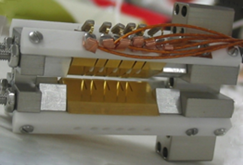
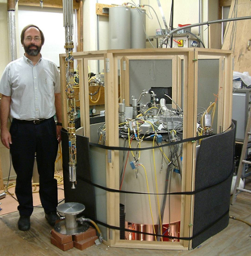
Figure 24: Gerald Gabrielse (left) is shown with the apparatus he used to make some of the most precise measurements of a single electron.
Source: © Gerald Gabrielse.
While the Heisenberg uncertainty principle predicts the scatter in the results for a single measurement, it does not limit the precision with which a physical property of a quantum mechanical object can be measured. One example is a dimensionless property of an electron called its g-factor. Quantum electrodynamics, the quantum mechanical theory of the electromagnetic field, predicts that this g-factor is almost, but not quite equal to 2. Gerald Gabrielse and his team at Harvard University used the apparatus shown here to confine an electron in a miniature cyclotron-like device. The actual device hangs suspended from a small refrigerator at the left of the apparatus. In operation, the refrigerator fits in a superconducting magnet in a low-temperature cryostat within the bulky housing. The result of the measurement was g/2 = 1.00115965218085, confirming the prediction of QED. The uncertainty in the measurement is 0.76 parts per trillion. (Unit: 5)

Myths about the uncertainty principle.

Heisenberg’s uncertainty principle is among the most widely misunderstood principles of quantum physics. Non-physicists sometimes argue that it reveals a fundamental shortcoming in science and poses a limitation to scientific knowledge. On the contrary, the uncertainty principle is seminal to quantum measurement theory, and quantum measurements have achieved the highest accuracy in all of science. It is important to appreciate that the uncertainty principle does not limit the precision with which a physical property, for instance a transition frequency, can be measured. What it does is to predict the scatter of results of a single measurement. By repeating the measurements, the ultimate precision is limited only by the skill and patience of the experimenter. Should there be any doubt about whether the uncertainty principle limits the power of precision in physics, measurements made with the apparatus shown in Figure 24 should put them to rest. The experiment confirmed the accuracy of a basic quantum mechanical prediction to an accuracy of one part in 10¹², one of the most accurate tests of theory in all of science.

The uncertainty principle and the world about us

Because the quantum world is so far from our normal experience, the uncertainty principle may seem remote from our everyday lives. In one sense, the uncertainty principle really is remote. Consider, for instance, the implications of the uncertainty principle for a baseball. Conceivably, the baseball could fly off unpredictably due to its intrinsically uncertain momentum. The more precisely we can locate the baseball in space, the larger is its intrinsic momentum. So, let’s consider a pitcher who is so sensitive that he can tell if the baseball is out of position by, for instance, the thickness of a human hair, typically 0.1 mm or 10^-4 m. According to the uncertainty principle, the baseball’s intrinsic speed due to quantum effects is about 10^-29 m/s. This is unbelievably slow. For instance, the time for the baseball to move quantum mechanically merely by the diameter of an atom would be roughly 20 times the age of the universe. Obviously, whatever might give a pitcher a bad day, it will not be the uncertainty principle.

Figure 25: The effect of quantum mechanical jitter on a pitcher, luckily, is too small to be observable.
Source: © Clive Grainger, 2010.
Can a baseball pitcher suffer from quantum mechanical jitter? According to the uncertainty principle, confining the baseball in the pitcher’s hand inevitably causes it to jitter. However, as the calculation shows, even if the ball is confined as tightly as the thickness of a hair, the time to see the effect of the jitter would be more than the age of the universe. Although baseball pitchers do not need to worry about quantum mechanical jitter, this zero-point motion can be significant in nano-mechanical devices. For instance, zero-point motion in the electromagnetic field, otherwise called “vacuum fluctuation,” gives rise to attractive forces between bodies, called “Casimir forces,” that can limit mechanical sensitivity. (Unit: 5)

Nevertheless, effects of the uncertainty principle are never far off. Our world is composed of atoms and molecules; and in the atomic world, quantum effects rule everything. For instance, the uncertainty principle prevents electrons from crashing into the nucleus of an atom. As an electron approaches a nucleus under the attractive Coulomb force, its potential energy falls. However, localizing the electron near the nucleus requires the sharpening of its wavefunction. This sharpening causes the electron’s momentum spread to get larger and its kinetic energy to increase. At some point, the electron’s total energy would start to increase. The quantum mechanical balance between the falling potential energy and rising kinetic energy fixes the size of the atom. If we magically turned off the uncertainty principle, atoms would vanish in a flash. From this point of view, you can see the effects of the uncertainty principle everywhere.

The discovery that laser light can cool atoms to less than a millionth of a degree above absolute zero opened a new world of quantum physics. Previously, the speeds of atoms due to their thermal energy were always so high that their de Broglie wavelengths were much smaller than the atoms themselves. This is the reason why gases often behave like classical particles rather than systems of quantum objects. At ultra-low temperatures, however, the de Broglie wavelength can actually exceed the distance between the atoms. In such a situation, the gas can abruptly undergo a quantum transformation to a state of matter called a Bose-Einstein condensate. The properties of this new state are described in Unit 6. In this section, we describe some of the techniques for cooling and trapping atoms that have opened up a new world of ultracold physics. The atom-cooling techniques enabled so much new science that the 1997 Nobel Prize was awarded to three of the pioneers: Steven Chu, Claude Cohen-Tannoudji, and William D. Phillips.

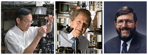
Figure 26: Recipients of the 1997 Nobel Prize, for laser cooling and trapping of atoms.
Source: © Left: Steven Chu, Stanford University; Middle: Claude Cohen-Tannoudji, Jean-Francois DARS, Laboratoire Kastler Brossel; Right: William D. Phillips, NIST.

Doppler cooling

As we learned earlier, a photon carries energy and momentum. An atom that absorbs a photon recoils from the momentum kick, just as you experience recoil when you catch a ball. Laser cooling manages the momentum transfer so that it constantly slows the atom’s motion, slowing it down. In absorbing a photon, the atom makes a transition from its ground state to a higher energy state. This requires that the photon has just the right energy. Fortunately, lasers can be tuned to precisely match the difference between energy levels in an atom. After absorbing a photon, an atom does not remain in the excited state but returns to the ground state by a process called spontaneous emission, emitting a photon in the process. At optical wavelengths, the process is quick, typically taking a few tens of nanoseconds. The atom recoils as it emits the photon, but this recoil, which is opposite to the direction of photon emission, can be in any direction. As the atom undergoes many cycles of absorbing photons from one direction followed by spontaneously emitting photons in random directions, the momentum absorbed from the laser beam accumulates while the momentum from spontaneous emission averages to zero.

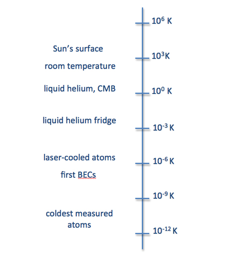
Figure 27: Temperature scale in physics
The scale in the above diagram is logarithmic, so each tick mark represents a temperature 1,000 times higher than the tick below it. On this scale, the difference between the Sun’s surface temperature and room temperature is a small fraction of the range of temperatures opened by the invention of laser cooling. The temperature of the first BECs was determined by watching the cloud of trapped atoms expand when the trap was turned off. At the coldest temperatures represented here, temperature is defined in terms of the energy contained in each degree of freedom of the atoms, including internal degrees of freedom. The so-called spin temperatures—based on the spin degree of freedom—of ultracold atoms have been measured down to 50 picokelvin. If we compare this diagram to Figure 21 of Unit 4, we see that the Planck scale of interest in high-energy physics is off the chart at 1032 K. (Unit: 5)

This diagram of temperatures of interest in physics uses a scale of factors of 10 (a logarithmic scale). On this scale, the difference between the Sun’s surface temperature and room temperature is a small fraction of the range of temperatures opened by the invention of laser cooling. Temperature is in the Kelvin scale at which absolute zero would describe particles in thermal equilibrium that are totally at rest. The lowest temperature measured so far by measuring the speeds of atoms is about 450 picokelvin (one picokelvin is 10^-12 K). This was obtained by evaporating atoms in a Bose-Einstein condensate.

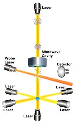
The process of photon absorption followed by spontaneous emission can heat the atoms just as easily as cool them. Cooling is made possible by a simple trick: Tune the laser so that its wavelength is slightly too long for the atoms to absorb. In this case, atoms at rest cannot absorb the light. However, for an atom moving toward the laser, against the direction of the laser beam, the wavelength appears to be slightly shortened due to the Doppler effect. The wavelength shift can be enough to permit the atom to absorb the light. The recoil slows the atom’s motion. To slow motion in the opposite direction, away from the light source, one merely needs to employ a second laser beam, opposite to the first. These two beams slow atoms moving along a single axis. To slow atoms in three dimensions, six beams are needed (Figure 28). This is not as complicated as it may sound: All that is required is a single laser and mirrors.

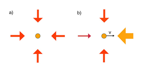
Figure 28: Red-detuned lasers don’t affect an atom at rest (left) but will slow an atom moving toward the light source (right).
Source: © Daniel Kleppner
Atoms moving with respect to a laser see light that is Doppler shifted. If an atom moves toward the light source, the light appears shifted to the blue. The laser must be tuned to the red side of an atomic resonance to be absorbed by the atom. Red-detuned lasers pointing along every axis can be used to slow down atoms in all directions, and thus cool them. If the atom is not moving, as shown on the left side of the diagram, the red-detuned lasers will not interact with the atom at all. If the atom is moving, however, it will absorb photons from the laser beam opposing its motion and slow down as the photon’s momentum is transferred to the atom. Cooling continues until the atom cannot detect the Doppler shift. This occurs when the Doppler shift becomes so small that it is masked by the natural linewidth of the atomic transition. (Unit: 5)

Laser light is so intense that an atom can be excited just as soon as it gets to the ground state. The resulting acceleration is enormous, about 10,000 times the acceleration of gravity. An atom moving with a typical speed in a room temperature gas, thousands of meters per second, can be brought to rest in a few milliseconds. With six laser beams shining on them, the atoms experience a strong resistive force no matter which way they move, as if they were moving in a sticky fluid. Such a situation is known as optical molasses.

As one might expect, laser cooling cannot bring atoms to absolute zero. The limit of Doppler cooling is actually set by the uncertainty principle, which tells us that the finite lifetime of the excited state due to spontaneous emission causes an uncertainty in its energy. This blurring of the energy level causes a spread in the frequency of the optical transition called the natural linewidth. When an atom moves so slowly that its Doppler shift is less than the natural linewidth, cooling comes to a halt. The temperature at which this occurs is known as the Doppler cooling limit. The theoretical predictions for this temperature are in the low millikelvin regime. However, by great good luck, it turned out that the actual temperature limit was lower than the theoretical prediction for the Doppler cooling limit. Sub-Doppler cooling, which depends on the polarization of the laser light and the spin of the atoms, lowers the temperature of atoms down into the microkelvin regime.

Atom traps

Like all matter, ultracold atoms fall in a gravitational field. Even optical molasses falls, though slowly. To make atoms useful for experiments, a strategy is needed to support and confine them. Devices for confining and supporting isolated atoms are called “atom traps.” Ultracold atoms cannot be confined by material walls because the lowest temperature walls might just as well be red hot compared to the temperature of the atoms. Instead, the atoms are trapped by force fields. Magnetic fields are commonly used, but optical fields are also employed.

Magnetic traps depend on the intrinsic magnetism that many atoms have. If an atom has a magnetic moment, meaning that it acts as a tiny magnet, its energy is altered when it is put in a magnetic field. The change in energy was first discovered by examining the spectra of atoms in magnetic fields and is called the Zeeman effect after its discoverer, the Dutch physicist Pieter Zeeman.

Because of the Zeeman effect, the ground state of alkali metal atoms, the most common atoms for ultracold atom research, is split into two states by a magnetic field. The energy of one state increases with the field, and the energy of the other decreases. Systems tend toward the configuration with the lowest accessible energy. Consequently, atoms in one state are repelled by a magnetic field, and atoms in the other state are attracted. These energy shifts can be used to confine the atoms in space.

The MOT

Figure 29: Atoms trapped in a MOT.
Source: © Martin Zwierlein.

The magneto-optical trap, or MOT, is the workhorse trap for cold atom research. In the MOT, a pair of coils with currents in opposite direction creates a magnetic field that vanishes at the center. The field points inward along the z-axis but outward along the x- and y-axes. Atoms in a vapor are cooled by laser beams in the same configuration as optical molasses, centered on the midpoint of the system. The arrangement by itself could not trap atoms because, if they were pushed inward along one axis, they would be pushed outward along another. However, by employing a trick with the laser polarization, it turns out that the atoms can be kept in a state that is pushed inward from every direction. Atoms that drift into the MOT are rapidly cooled and trapped, forming a small cloud near the center.

To measure the temperature of ultracold atoms, one turns off the trap, letting the small cloud of atoms drop. The speeds of the atoms can be found by taking photographs of the ball and measuring how rapidly it expands as it falls. Knowing the distribution of speeds gives the temperature. It was in similar experiments that atoms were sometimes found to have temperatures below the Doppler cooling limit, not in the millikelvin regime, but in the microkelvin regime. The reason turned out to be an intricate interplay of the polarization of the light with the Zeeman states of the atom causing a situation known as the Sisyphus effect. The experimental discovery and the theoretical explanation of the “Sisyphus effect” were the basis of the Nobel Prize to Chu, Cohen-Tannoudji, and Phillips in 1997.

Evaporative cooling

When the limit of laser cooling is reached, the old-fashioned process of evaporation can cool a gas further. In thermal equilibrium, atoms in a gas have a broad range of speeds. At any instant, some atoms have speeds much higher than the average, and some are much slower. Atoms that are energetic enough to fly out of the trap escape from the system, carrying away their kinetic energy. As the remaining atoms collide and readjust their speeds, the temperature drops slightly. If the trap is slowly adjusted so that it gets weaker and weaker, the process continues and the temperature falls. This process has been used to reach the lowest kinetic temperatures yet achieved, a few hundred picokelvin. Evaporative cooling cannot take place in a MOT because the constant interaction between the atoms and laser beams keeps the temperature roughly constant. To use this process to reach temperatures less than a billionth of a degree above absolute zero, the atoms are typically transferred into a trap that is made purely of magnetic fields.

Optical traps

Atoms in light beams experience forces even if they don’t actually absorb or radiate photons. The forces are attractive or repulsive depending on whether the laser frequency is below or above the transition frequency. These forces are much weaker than photon recoil forces, but if the atoms are cold enough, they can be large enough to confine them. For instance, if an intense light beam is turned on along the axis of a MOT that holds a cloud of cold atoms, the MOT can be turned off, leaving the atoms trapped in the light beam. Unperturbed by magnetic fields or by photon recoil, for many purposes, the environment is close to ideal. This kind of trap is called an optical dipole trap.

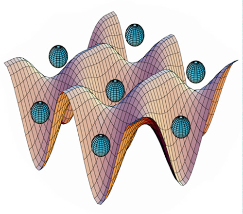
Figure 30: Atoms trapped in an optical lattice.
Source: © NIST.
The egg-carton-like structure shown here represents the energy landscape an atom experiences in an optical lattice. Atoms are attracted to the low-energy regions, which correspond to regions where the optical field is strong. An optical lattice similar to this was used to hold the atoms in the rectangular array in Figure 2. Lattices can be designed to confine atoms in one, two or three dimensions, making it possible to study different types of many-body structures. Furthermore, the beams can be controlled to provide geometries not normally found in nature, for instance a triangular lattice. (Unit: 5)

If the laser beam is reflected back on itself to create a standing wave of laser light, the standing wave pattern creates a regular array of areas where the optical field is strong and weak known as an optical lattice. Atoms are trapped in the regions of the strong field. If the atoms are tightly confined in a strong lattice and the lattice is gradually made weaker, the atoms start to tunnel from one site to another. At some point the atoms move freely between the sites. The situation is similar to the phase transition in a material that abruptly turns from an insulator into a conductor. This is but one of many effects that are well known in materials and can now be studied using ultracold atoms that can be controlled and manipulated with a precision totally different from anything possible in the past.

Why the excitement?

The reason that ultracold atoms have generated enormous scientific excitement is that they make it possible to study basic properties of matter with almost unbelievable clarity and control. These include phase transitions to exotic states of matter such as superfluidity and superconductivity that we will learn about in Unit 8, and theories of quantum information and communication that are covered in Unit 7. There are methods for controlling the interactions between ultracold atoms so that they can repel or attract each other, causing quantum changes of state at will. These techniques offer new inroads to quantum entanglement—a fundamental behavior that lies beyond this discussion—and new possibilities for quantum computation. They are also finding applications in metrology, including atomic clocks.

The words “Atomic Clock” occasionally appear on wall clocks, wristwatches, and desk clocks, though in fact none of these devices are really atomic. They are, however, periodically synchronized to signals broadcast by the nation’s timekeeper, the National Institute of Standards and Technology (NIST). The NIST signals are generated from a time scale controlled by the frequency of a transition between the energy states of an atom—a true atomic clock. In fact, the legal definition of the second is the time for 9,192,631,770 cycles of a particular transition in the atom ¹³³Cs.

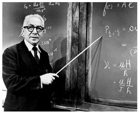
Figure 31: Isidor Isaac Rabi pioneered atomic physics in the U.S. during the 1930s, invented magnetic resonance, and first suggested the possibility of an atomic clock.
Source: © Trustees of Columbia University in the City of New York.
The lower portion of the blackboard shows Rabi’s calculation for the transition frequency in a magnetic resonance experiment. Rabi, an Austrian-born physicist who spent most of his career at Columbia University, received the 1944 Nobel Prize in Physics for developing the resonance method of recording the magnetic properties of atomic nuclei. This technique has broad-ranging applications from medical imaging to atomic clocks. (Unit: 5)

Columbia University physicist Isidor Isaac Rabi first suggested the possibility that atoms could be used for time keeping. Rabi’s work with molecular beams in 1937 opened the way to broad progress in physics, including the creation of the laser as well as nuclear magnetic resonance, which led to the MRI imaging now used in hospitals. In 1944, the same year he received the Nobel Prize, he proposed employing a microwave transition in the cesium atom, and this system has been used ever since. The first atomic clocks achieved an accuracy of about 1 part in 10¹⁰. Over the years, their accuracy has been steadily improved. Cesium-based clocks now achieve accuracy greater than 1 part in 10¹⁵, 10,000 times more accurate than their predecessors, which is generally believed to be close to their ultimate limit. Happily, as will be described, a new technology for clocks based on optical transitions has opened a new frontier for precision.

A clock is a device in which a motion or event occurs repeatedly and which has a mechanism for keeping count of the repetitions. The number of counts between two events is a measure of the interval between them, in units of the period of the atomic transition frequency. If a clock is started at a given time—that is, synchronized with the time system—and kept going, then the accumulated counts define the time. This statement actually encapsulates the concept of time in physics.

In a pendulum clock, the motion is a swinging pendulum, and the counting device is an escapement and gear mechanism that converts the number of swings into the position of the hands on the clock face. In an atomic clock, the repetitious event is the quantum mechanical analogy to the physical motion of an atom: the frequency for a transition between two atomic energy states. An oscillator is adjusted so that its frequency matches the transition frequency, effectively making the atom the master of the oscillator. The number of oscillation cycles—the analogy to the number of swings of a pendulum—is counted electronically.

The quality of a clock—essentially its ability to agree with an identical clock—depends on the intrinsic reproducibility of the periodic event and the skill of the clockmaker in counting the events. A cardinal principle in quantum mechanics is that all atoms of a given species are absolutely identical. Consequently, any transition frequency could form the basis for an atomic clock. The art lies in identifying the transition that can be measured with the greatest accuracy. For this, a high tick rate is desirable: It would be difficult to compare the rates of two clocks that ticked, for instance, only once a month. As the definition of the second reveals, cesium-based clocks tick almost 10 billion times per second.

Atomic clocks and the uncertainty principle

The precision with which an atomic transition can be measured is fundamentally governed by the uncertainty principle. As explained in Section 6, because of the time-energy uncertainty principle, there is an inherent uncertainty in the measurement of a frequency (which is essentially an energy) that depends on the length of the time interval during which the measurement is made. To reduce the uncertainty in the frequency measurement, the observation time should be as long as possible.

Figure 32: Schematic diagram of an atomic fountain clock.
Source: © NIST/Jeffrey Aarons.
The first step in creating an atomic fountain is to trap and cool the atoms using the techniques described in the previous section. Once a cloud of cold atoms is trapped in the region where the six laser beams overlap, the trap lasers are turned off. Two vertical laser beams are then pulsed on and off to give the atoms a gentle upward push. The ball of atoms rises about a meter before it begins to fall under the influence of gravity. As they do this, the atoms pass through a microwave cavity twice: once on the way up, and once on the way down. Depending on the microwave frequency in the cavity, the state of the atoms might be altered as they interact with the microwave signal. If the microwave frequency is perfectly matched to the atoms, the atoms will emit light after interacting with the probe laser beam below the microwave cavity. This light is collected by the detector and the frequency of the microwave cavity is adjusted to maximize the signal on the detector. Once linked to the atomic resonance, the microwave frequency is a periodic signal that can be used for timekeeping just like the pendulum in a grandfather clock. (Unit: 5)

In an atomic clock, the observation time is the time during which the atoms interact with the microwave radiation as they make the transition. Before the advent of ultracold atoms and atom trapping, this time was limited by the speed of the atoms as they flew through the apparatus. However, the slow speed of ultracold atoms opened the way for new strategies, including the possibility of an atomic fountain. In an atomic fountain, a cloud of cold atoms is thrust upward by a pulse of light. The atoms fly upward in the vacuum chamber, and then fall downward under the influence of gravity. The observation time is essentially the time for the atoms to make a roundtrip. For a meter-high fountain, the time is about one second.

The quality of an atomic clock depends on how well it can approach ideal measurement conditions. This requires understanding and controlling the many sources of error that can creep in. Errors arise from noise in the measurement process, perturbations to the atomic system by magnetic fields and thermal (blackbody) radiation, energy level shifts due to interactions between the atoms, and distortions in the actual measurement process. The steady improvement in the precision of atomic clocks has come from incremental progress in identifying and controlling these effects.

The cesium fountain clock

The cesium clock operates on a transition between two energy states in the electronic ground state of the atom. As mentioned in Section 7, the ground state of an alkali metal atom is split into two separate energy levels in a magnetic field. Even in the absence of an external magnetic field, however, the ground state is split in two. This splitting arises from a magnetic interaction between the outermost in the atom electron and the atom’s nucleus, known as the hyperfine interaction. The upper hyperfine state can in principle radiate to the lower state by spontaneous emission, but the lifetime for this is so long—thousands of years—that for all purposes, both states are stable. The transition between these two hyperfine states is the basis of the cesium clock that defines the second.

The cesium fountain clock operates in a high vacuum so that atoms move freely without colliding. Cesium atoms from a vapor are trapped and cooled in a magneto-optical trap. The trap lasers both cool the atoms and “pump” them into one of the hyperfine states, state A. Then, the wavelength of the trap laser beam pointing up is tuned to an optical transition in the atoms, giving the cloud a push by photon recoil. The push is just large enough to send the atoms up about one meter before they fall back down. The atoms ascend through a microwave cavity, a resonant chamber where the atoms pass through the microwave field from an oscillator. The field is carefully controlled to be just strong enough that the atoms make “half a transition,” which is to say that if one observed the states of the atoms as they emerged from the cavity, half would be in hyperfine state A and half would be in state B. Then the atoms fly up, and fall back. If the frequency is just right, the atoms complete the transition as they pass through the cavity, so that they emerge in state B. The atoms then fall through a probe laser, which excites only those that are in state B. The fluorescence of the excited atoms is registered on a detector. The signal from the detector is fed back to control the frequency of the microwave oscillator, so as to continuously stay in tune with the atoms.

Figure 33: This apparatus houses the NIST F1 cesium fountain clock, which is the primary time and frequency standard of the United States.
Source: © NIST.
This apparatus, found in the NIST physics laboratory in Boulder, Colorado, houses the primary time and frequency standard of the United States. It is an atomic fountain clock that makes use of two hyperfine levels in the ground state of cesium atoms to define the second. The fountain rises and falls within the vertical cylinder at the top of the image. The optical table and electronics rack to the right of the table contain the laser beams and microwave electronics needed to operate the clock. The uncertainty in the clock frequency is about 5 x 10-16, which corresponds to a gain or loss of about 1 second in 60 million years! (Unit: 5)

If we plot the signal on the detector against the frequency of the oscillator, we end up with what is known as a resonance curve. The pattern, called a Ramsey resonance curve, looks suspiciously like two-slit interference. In fact, it is an interference curve, but the sources interfere not in space but in time. There are two ways for an atom to go to state B from state A: by making the transition on the way up or on the way down. The final amplitude of the wavefunction has contributions from both paths, just as the wavefunction in two-slit interference has contributions from paths going through each of the slits. This method of observing the transition by passing the atom through a microwave field twice is called the “separated oscillatory field method” and its inventor, Norman F. Ramsey, received the Nobel Prize for it in 1989.

Optical clocks

A useful figure of quality for atomic clocks is the ratio of its frequency  to the uncertainty in its frequency, Δv. For a given value of Δv, the higher the frequency, the better the clock. With atom-cooling techniques, there are many possibilities for keeping atoms close to rest so that Δv is small. Consequently, clocks operating at optical frequencies, in the petahertz (10¹⁵ Hz) region, are potentially much more accurate than cesium-based clocks that operate in the gigahertz (10⁹ Hz) region. However, two impediments have delayed the advent of optical clocks. Fortunately, these have been overcome, and optical clock technology is moving forward rapidly.

The first impediment was the need for an incredibly stable laser to measure the atomic signal. In order to obtain a signal from the atoms, the laser must continue oscillating smoothly on its own during the entire time the atoms are being observed. The requirement is formidable: a laser oscillating at a frequency of close to 10¹⁵ Hz that fluctuates less than 1 Hz. Through a series of patient developments over many years, this challenge has been met.

The second impediment to optical clocks was the problem of counting cycles of light. Although counting cycles of an oscillating electric field is routine at microwave frequencies using electronic circuitry, until recently there was no way to count cycles at optical frequencies. Fortunately, a technology has been invented. Known as the “frequency comb,” the invention was immediately recognized as revolutionary. The inventors, Theodor W. Hänsch and John L. Hall, were awarded the Nobel Prize in 2005 “for their contributions to the development of laser-based precision spectroscopy including the optical frequency-comb technique.”

Figure 34: The heart of a next-generation optical clock.
Source: © Ion Storage Group, NIST
The next generation of atomic clocks will operate at optical frequencies. Such clocks are in the laboratory stage now, but one can expect that they will become practical devices in the coming years. Two quite different approaches are employed, both based on laser-cooled particles. The first, shown here, employs a single trapped ion. This trap holds a second ion for support purposes, but the frequency reference is a single ion that is held in almost ideal conditions of isolation. The second approach employs a cloud of ultracold atoms held in an optical lattice, such as those shown in Figure 2 (Unit 5, Section 1). The clock has the disadvantage that the lattice can perturb the atoms, and the atoms can perturb each other. However, it has the advantage of providing large signals and operating continuously. At the moment, the two approaches are running almost neck-and-neck. (Unit: 5)

Optical clocks are only in the laboratory stage but progress is rapid. One type of clock employs ions stored in electromagnetic traps, similar to the trap used in Figure 1; another employs neutral atoms confined in an optical lattice such as in Figure 2. Figure 34 shows a state-of-the-art ion-based clock at NIST. A pair of such clocks has recently demonstrated a relative accuracy greater than one part in 10¹⁷. Making these clocks into practical devices is an interesting engineering challenge.

In the new world of precise clocks, transmitting timing signals and comparing clocks in different locations presents a major challenge. Transmissions through the atmosphere or by a satellite relay suffer bad atmospheric fluctuations. The signals can be transmitted over optical fibers, but fibers can introduce timing jitter from vibrations and optical nonlinearities. These can be overcome for distances of tens of kilometers by using two-way monitoring techniques, but methods for extending the distances to thousands of kilometers have yet to be developed. However, there is an even more interesting impediment to comparing clocks at different locations. The gravitational redshift explained in Unit 3 changes the rates of clocks by 1 part in 10¹⁶ for each meter of altitude, near Earth’s surface. Clocks are approaching the regime of parts in 10¹⁸. To compare clocks in different locations, the relative altitudes would need to be known to centimeters. Earth’s surface is constantly moving by tens of centimeters due to tides, weather, and geological processes. This presents not merely a practical problem but also a conceptual problem, for it forces us to realize that time and gravity are inextricably interlinked. Because of this, the view that time is essentially the clicks on a clock begins to seem inadequate.

Payoffs from basic research

When Isidor Isaac Rabi proposed the possibility of an atomic clock, he had a scientific goal in mind: to observe the effect of gravity on time—the gravitational redshift—predicted by Einstein’s theory of general relativity. The quest to confirm Einstein’s prediction motivated the field. Today, the gravitational redshift has not only been observed, but also measured to high precision. However, the biggest impacts of atomic clocks were totally unforeseen. Global Positioning System (GPS) is one of these.

The GPS is a network of satellites positioned so that several of them are essentially always in view. A receiver calculates its location from information transmitted by the satellites about their time and position at each instant. The satellites carry one or more atomic clocks whose times are periodically updated by a master atomic clock in a ground station. The GPS system is a miracle of engineering technology: sophisticated satellites, integrated electronics and advanced communications, information processing, geodesy, and orbital mechanics. But without atomic clocks, there would be no GPS. Furthermore, with the precision inherent in the GPS system, the gravitational redshift is not only detectable, but to overlook it would cause catastrophic navigational errors.

Figure 35: This VLBI image of jets from a black hole could not have been produced without atomic clocks.
Source: © Steven Tingay, Curtin University, Australia
This image, taken using Very Long Baseline Interferometry (VLBI) shows relativistic jets produced by a black hole nearly 10 million light-years from our galaxy. The black hole is at the lower end of the bright linear structure, where the emission intensity is highest. One of the bi-directional jets is ejected to the top left of the image. The opposing jet is ejected to the lower right of the image. The jet to the lower right is receding from us and is therefore much fainter than the jet to the upper left, which is approaching us. This is among the highest resolution images ever achieved in astronomy. Its literally astronomical resolution is made possible by employing atomic clocks at each globally spaced radio observatory that compose the interferometer system. (Unit: 5)

Atomic clocks have applications in fundamental science as well. The technique of very long baseline radio interferometry (VLBI) permits Earth to be converted to a giant radio telescope. Signals from radio observatories on different continents can be brought together and compared to provide the angular resolution of an Earth-sized dish. To do this, however, the astronomical radio signals must first be recorded against the signal from an atomic clock. The records are then brought together and their information is correlated. VLBI can reveal details less than a millionth of a degree, the highest resolution achieved in all of astronomy.

Although Einstein’s theory of gravity is one of the most abstract subjects in science, the search to study it led to the invention of GPS and the creation of VLBI. This history illustrates, if illustration is needed, that the pursuit of basic knowledge is a worthy goal for scientists and a wise investment for society.

The paradox of how a wave can be a particle and a particle can be a wave was brought up in Section 4, but not resolved. The issue is far from trivial and was fiercely debated in the early days of quantum mechanics. Niels Bohr even designed a hypothetical experiment to clarify the question of whether you could detect which slit a photon passed through in a two-slit interference experiment. For light to interfere, it must slightly change its direction as it passes through a slit in order to merge with the second beam.

Consequently, passing through a slit must slightly alter a photon’s direction, which means that the slit has altered the photon’s momentum. The photon must give an opposite momentum to the slit. Bohr’s apparatus was designed to detect the recoil of the slit. If this were possible, an observer could decide which slit each photon passed through in creating an interference pattern, revealing both the particle and wave nature of light simultaneously. However, Bohr proved that detecting the photon would actually wipe out the interference pattern.

Thinking about waves passing through slits provides a different way to understand the situation. The waves might be light waves but they could just as well be matter waves. As the waves emerge from the slits, they diverge in a diffraction pattern. The wave intensity on the viewing screen might be registered on a camera, as in Figure 11, or measured by detections with particle counters, creating images similar to those in Figure 15. For the sake of discussion, we assume that the individual atoms or photons are detected with particle counters.

If the slits are close together, the diffraction patterns of particles coming through them overlap. In time the counts add to give a two-slit interference pattern, which is the signature of waves. What about the intermediate case? If the slits are far enough apart that the diffraction patterns only overlap a little bit, we should be able to place two detectors that only see particles passing through one or the other of the slits, and a detector in the center that sees two-slit interference. The conclusion is that if one knows from which of two slits the signal arises, one must ascribe the signal to the arrival of a particle. However, if there is no way to distinguish which of two possibilities gave rise to the signal, one must ascribe the signal to the arrival of waves.

Figure 36: The two-slit interference pattern depends on the distance between the slits.
Source: © Daniel Kleppner.
If two slits are spaced far enough apart (left), no interference pattern appears on the screen. If the two slits are close together (center), the interference pattern we’ve seen throughout this unit appears. However, if the slits are placed an intermediate distance apart (right), there is a region where the diffraction patterns overlap, and a region in which they do not overlap. In this third case, you can observe either the wave nature or the particle nature of light, depending on where you place your detector. (Unit: 5)

The answer to the question, “Is light composed of waves or particles?” is “Both.” If you search for light’s wave properties, you will find them. If you search for light’s particle properties, you will find them, too. However, you cannot see both properties at the same time. They are what Bohr called complementary properties. One needs both properties for a complete understanding of light, but they are fundamentally incompatible and cannot be observed at the same time. Thus, the wave-particle paradox presents a contradiction that is not really true, but merely apparent.

We have discussed the wave-particle paradox for light, but the same reasoning applies to atoms and matter waves. Atoms are waves and they are particles, but not at the same time. You will find what you look for.

• Rainer Blatt and David Wineland, “Entangled states of trapped atomic ions,” Nature, June 2008, p. 1008.
• Steven Chu, Claude Cohen-Tannoudji, and William D. Phillips: Nobel Prize Lectures, available at http://nobelprize.org/nobel_prizes/physics/laureates/1997/.
• Albert Einstein, “Einstein’s Essays in Science,” Dover Publications (2009).
• Tony Jones, “Splitting the Second: The Story of Atomic Time,” Taylor and Francis (2008).

Momentum and Energy

The momentum has the value p = h/λ = hnL/2. The energy of the particle, E, is its kinetic energy, p²/2M, and it follows that the energy of the n^th state is E_n=n²(hL)²/8M.