


Physics for the 21st Century
Manipulating Light Online Textbook
Online Text by Lene Hau
The videos and online textbook units can be used independently. When using both, it is possible to start with either one. Watching the video first, and then reading the unit from the online textbook is recommended.
Each unit was written by a prominent physicist who describes the cutting edge advances in his or her area of research and the potential impacts of those advances on everyday life. The classical physics related to each new topic is covered briefly to help the reader better understand the research, its effects, and our current understanding of physics.
Click on “Content By Unit” (in the menu to the left) and select a unit title to view the Web version of the online text, which includes links to related material. Or, download PDF versions of the units below.
1. Introduction

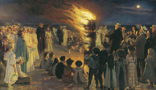
Figure 1: Saint Hans bonfire—Midsummer celebration in Skagen, Denmark.
Source: Painting by P.S. Krøyer: Sct. Hans-blus på Skagen, 1906; owned by Skagen Museum.
The celebration of the summer solstice in Denmark dates back to pagan times, but became known as Saint Hans (Saint John’s Eve) after the arrival of Christianity. The painting is by P.S. Krøyer, a famous Danish painter who was part of the community of painters in Skagen at the turn of the 20th century. Skagen is an old fishing village at the very northern-most tip of the European continent where Skagerak strait meets the North Sea. Painters viewed the light at Skagen as being very special and hence chose to live and paint there. The most unusual lighting of all is the lighting around midsummer, when the sun doesn’t set until 10:30 p.m. and rises again at 3 a.m. In between it is not really dark; rather there is a metallic-blue night sky. This special lighting makes midsummer a very special time of year. (Unit: 7)
Light has fascinated humans for thousands of years. In ancient times, summer solstice was a celebrated event. Even to this day, the midsummer solstice is considered one of the most important events of the year, particularly in the northern-most countries where the contrast between the amount of light in summer and winter is huge. Visible daylight is intense due to the proximity of the Earth to the Sun. The Sun is essentially a huge nuclear reactor, heated by the energy released by nuclear fusion. When something is hot, it radiates. The surface of the Sun is at a temperature of roughly 6000 K (roughly 10,000°F). Our eyes have adapted to be highly sensitive to the visible wavelengths emitted by the Sun that can penetrate the atmosphere and reach us here on Earth. The energy carried in sunlight keeps the Earth at a comfortable temperature and provides the energy to power essentially everything we do through photosynthesis in plants, algae, and bacteria—both the processing happening right now as well as what took place millions of years ago to produce the energy stored in fossil fuels: oil, gas, and coal.
The interaction of light with different substances has long been a subject of great interest, both for basic science and for technological applications. The manipulation of light with engineered materials forms the basis for much of the technology around us, ranging from eyeglasses to fiber-optic cables. Many of these applications rely on the fact that light travels at different speeds in different materials.
The speed of light, therefore, plays a special role that spans many aspects of physics and engineering. Understanding and exploiting the interaction between light and matter, which govern the speed of light in different media, are topics at the frontier of modern physics and applied science. The tools and techniques employed to explore the subtle and often surprising interplay between light and matter include lasers, low-temperature techniques (cryogenics), low-noise electronics, optics, and nanofabrication.

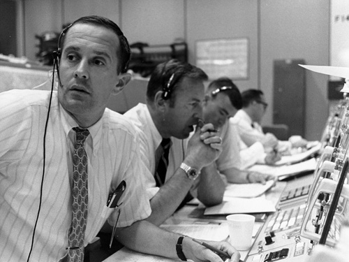
Figure 2: Flight controllers Charles Duke (Capcom), Jim Lovell (backup CDR), and Fred Haise (backup LMP) during lunar module descent.
Source: © NASA.
The finite speed of light took its toll on the Apollo astronauts, who had to wait 2.5 seconds to hear transmissions from flight controllers Charles Duke and Jim Lovell, pictured here. (Unit: 7)
Light travels fast, but not infinitely fast. It takes about two and a half seconds for a pulse of light to make the roundtrip to the Moon and back. When NASA’s ground control station was engaged in discussions with the Apollo astronauts at the Moon, the radio waves carrying the exchange traveled at light speed. The 2.5 second lag due to the radio waves moving at the finite speed of light produced noticeable delays in their conversations. Astronomers measure cosmic distances in terms of the time it takes light to traverse the cosmos. A light-year is a measure of distance, not time: it’s the length that light travels in a year. The closest star to the Sun is about four light-years away. For more down-to-Earth separations, a roundtrip at light speed from London to Los Angeles would take about 0.06 seconds.
So, if the upper limit to the speed of light is c, an astonishing 300 million meters per second (186,000 miles per second), how much can we slow it down? Light traveling in transparent materials moves more slowly than it does in a vacuum, but not by much. In air, light travels about 99.97% as fast as it does in a vacuum. The index of refraction, n, of a material is the ratio between light’s speed in empty space relative to its speed in the material. In a typical glass (n = 1.5), the light is traveling about 67% as fast as it does in a vacuum. But can we do better? Can we slow light down to human speeds? Yes!
This unit explores the fascinating quest for finding ways to slow down and even stop light in the laboratory. Perhaps this extreme limit of manipulating light in materials could give rise to novel and profound technological applications.
2. Measuring and Manipulating the Speed of Light
Interest in studying light, and in measuring its speed in different circumstances, has a long history. Back in the 1600s, Isaac Newton thought of light as consisting of material particles (corpuscles). But Thomas Young’s experiments showed that light can interfere like merging ripples on a water surface. This vindicated Christiaan Huygens’ earlier theory that light is a wave. Quantum mechanics has shown us that light has the properties of both a particle and a wave, as described in Unit 5.
Scientists originally believed that light travels infinitely fast. But in 1676, Ole Rømer discovered that the time elapsed between eclipses of Jupiter’s moons was not constant. Instead, the period varied with the distance between Jupiter and the Earth. Rømer could explain this by assuming that the speed of light was finite. Based on observations by Michael Faraday, Hans Christian Ørsted, André-Marie Ampère, and many others in the 19th century, James Clerk Maxwell explained light as a wave of oscillating electric and magnetic fields that travels at the finite speed of 186,000 miles per second, in agreement with Rømer’s observations.

Figure 3: The biker wins the race against the light pulse!
Source: © John Newman and Lene V. Hau.
In this unit, we describe how light can be slowed to below the speed of a bicycle, and how it can be stopped altogether. Even weirder: we can convert light to matter and back to light with no loss of information. (Unit: 7)
Experiments on the speed of light continued. Armand Hippolyte Fizeau was the first to determine the light speed in an Earth-based experiment by sending light through periodically spaced openings in a fast rotating wheel, then reflecting the light in a mirror placed almost 10 km away. When the wheel rotation was just right, the reflected light would again pass through a hole in the wheel. This allowed a measurement of the light speed. Fizeau’s further experiments on the speed of light in flowing water, and other experiments with light by Augustin-Jean Fresnel, Albert Michelson, and Edward Morley, led Albert Einstein on the path to the theory of special relativity. The speed of light plays a special role in that theory, which states that particles and information can never move faster than the speed of light in a vacuum. In other words: the speed of light in a vacuum sets an absolute upper speed limit for everything.
Bending light with glass: classical optics
The fact that light travels more slowly in glass than in air is the basis for all lenses, ranging from contact lenses that correct vision to the telephoto lenses used to photograph sporting events. The phenomenon of refraction, where the direction that a ray of light travels is changed at an interface between different materials, depends on the ratio of light’s speed in the two media. This is the basis for Snell’s Law, a relationship between the incoming and outgoing ray angles at the interface and the ratio of the indices of refraction of the two substances.
By adjusting the curvature of the interface between two materials, we can produce converging and diverging lenses that manipulate the trajectory of light rays through an optical system. The formation of a focused image, on a detector or on a screen, is a common application. In any cell phone, the camera has a small lens that exploits variation in the speed of light to make an image, for example.
If different colors of light move at different speeds in a complex optical system, the different colors don’t traverse the same path. This gives rise to “chromatic aberration,” where the different colors don’t all come to the same focus. The difference in speed with a wavelength of light also allows a prism to take an incoming ray of white light that contains many colors and produce beams of different colors that emerge at different angles.
Finding breaks in optical fibers: roundtrip timing

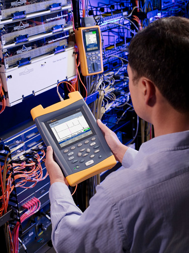
Figure 4: An optical time domain reflectometer in use.
Source: © Wikimedia Commons, Creative Commons Attribution-Share Alike 3.0. 25 September 2009
This optical time domain reflectometer is being used to characterize an optical fiber by injecting a series of optical pulses and measuring backscattered light. These devices make use of the finite speed of light to measure the overall length of a fiber, as well as the distance to any breaks or imperfections. (Unit: 7)
A commercial application of the speed of light is the Optical Time Domain Reflectometer (OTDR). This device sends a short pulse of light into an optical fiber, and measures the elapsed time and intensity of any light that comes back from the fiber. A break in the fiber produces a lot of reflected light, and the elapsed time can help determine the location of the problem. Even bad joints or poor splices can produce measurable reflections, and can also be located with OTDR. Modern OTDR instruments can locate problems in optical fiber networks over distances of up to 100 km.
The examples given above involve instances where the light speeds in materials and in a vacuum aren’t tremendously different, hardly changing by a factor of two. Bringing the speed of light down to a few meters per second requires a different approach.
3. A Sound Design for Slowing Light
Our objective is to slow light from its usual 186,000 miles per second to the speed of a bicycle. Furthermore, we can show that light can be completely stopped, and even extinguished in one part of space and regenerated in a completely different location.
To manipulate light to this extreme, we first need to cool atoms down to very low temperatures, to a few billionths of a degree above absolute zero. As we cool atoms to such low temperatures, their quantum nature becomes apparent: We form Bose-Einstein condensate and can get millions of atoms to move in lock-step—all in the same quantum state as described in Units 5 and 6.
Atom refrigerator
Achieving these low temperatures requires more than the use of a standard household refrigerator: We need to build a special atom refrigerator.

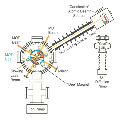
Figure 5: Sketch of experimental setup used to create ultracold atoms.
Source: © Brian Busch and Lene Hau.
This sketch of an atom refrigerator shows the atom source (“candlestick” atomic beam source), the atom slower, and the optical molasses which is created in the main vacuum chamber by three pairs of counterpropagating laser beams (MOT beams; the third laser beam pair goes in and out of the plane of the sketch). The electromagnet (“Dee” magnet) is used to hold the laser-cooled atoms in place during their further cooling to nanokelvin temperatures where Bose-Einstein condensates start to form. (Unit: 7)
In the setup we use in our laboratory, most parts have been specially designed and constructed. This includes the first stage of the cooling apparatus: the atom source. We have named it the “candlestick atomic beam source” because it works exactly like a candle. We melt a clump of sodium metal that we have picked from a jar where it is kept in mineral oil. Sodium from the melted puddle is then delivered by wicking (as in a candle) to a localized hot spot that is heated to 650°F and where sodium is vaporized and emitted. To create a well-directed beam of sodium atoms, we send them through a collimation hole. The atoms that are not collimated are wicked back into the reservoir and can be recycled.

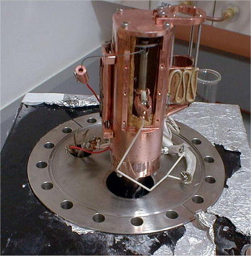
Figure 6: The atom source in the experimental setup is specially designed and called the “candlestick atomic beam source.”
Source: © Hau Laboratory.
Like most of the rest of the experimental apparatus, the atom source is specially designed and machined. The candlestick itself is a small molybdenum cylinder filled with stainless steel wire mesh and placed inside a copper pot. Wicking action on the mesh allows the delivery of melted sodium to the source emission point of the candlestick, a localized hot spot placed several centimeters above a reservoir of melted sodium at the bottom of the pot, and kept at the melting point for sodium. The copper pot has a collimation hole, and un-collimated sodium atoms are transported back to the reservoir and then wicked back up to the emission point. In the figure the source is shown from the rear and the candlestick is seen as the narrow gray cylinder in the sliced opening of the copper pot. The whole structure is mounted on a stainless steel vacuum flange. (Unit: 7)
This atom source produces a high-flux collimated beam of atoms—there is just one problem: The atoms come out of the source with a velocity of roughly 1500 miles per hour, which is much too fast for us to catch them. Therefore, we hit the atoms head-on with a yellow laser beam and use radiation pressure from that laser beam to slow the atoms. By tuning the frequency of the laser to a characteristic frequency of the atoms, which corresponds to the energy difference between energy levels in the atom (we say the laser is resonant with the atoms), we can get strong interactions between the laser light and the atoms. We use a laser beam with a power of roughly 50 mW (a typical laser pointer has a power of 1 mW), which we focus to a small spot at the source. This generates a deceleration of the atoms of 100,000 g’s, in other words 100,000 times more than the acceleration in the Earth’s gravitational field. This is enormous; and in a matter of just a millisecond (one-thousandth of a second) —and over a length of one meter—we can slow the atoms to 100 miles per hour.
Optical molasses
At this point, we can load the atoms efficiently into an optical molasses created in the middle of a vacuum chamber by three pairs of counter-propagating laser beams. These laser beams are tuned to a frequency slightly lower than the resonance absorption frequency, and we make use of the Doppler effect to cool the atoms. The Doppler effect is familiar from everyday life: A passing ambulance will approach you with the siren sounding at a high pitch; and as the ambulance moves away, the siren is heard at a much lower pitch. Moving atoms bombarded from all sides with laser beams will likewise see the lasers’ frequency shifted: If an atom moves toward the source of a laser beam, the frequency of the laser light will be shifted higher and into resonance with the atom; whereas for atoms moving in the same direction as the laser beam, the atoms will see a frequency that is shifted further from resonance. Therefore, atoms will absorb light—or photons—from the counter-propagating beams more than from the co-propagating beams; and since an atom gets a little momentum kick in the direction of the laser beam each time it absorbs a photon, the atoms will slow down. In this way, the laser beams create a very viscous medium—hence the name “optical molasses” in which the atoms will slow and cool to a temperature just a few millionths of a degree above absolute zero. We can never reach absolute zero (at -273°C or -460°F), but we can get infinitely close.

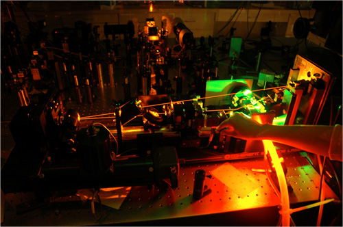
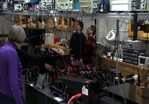
Figure 7: Running the experimental setup requires great focus.
The image shows first-year graduate student Jon Welsh and postdoctoral fellow Rui Zhang on the far side of the optics table, and Lene Hau is in the front. They are checking and discussing the performance of the feedback system for the laser frequency lock. (Unit: 7)
It may be surprising that lasers can cool atoms since they are also being used for welding, in nuclear fusion research, and for other high-temperature applications. However, a laser beam consists of light that is incredibly ordered. It has a very particular wavelength or frequency and propagates in a very particular direction. In laser light, all the photons are in lock-step. By using laser beams, we can transfer heat and disorder from the atoms to the radiation field. In the process, the atoms absorb laser photons and spontaneously re-emit light in random directions: The atoms fluoresce. Figure 7 shows a view of the lab during the laser cooling process. Figure 8 shows the optical table in daylight: As seen, many manhours have gone into building this setup.

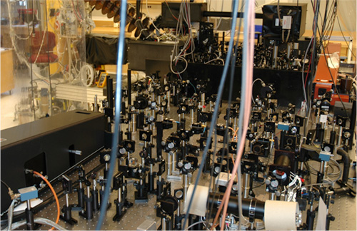
Figure 8: A view of the optics table.
Source: © Hau Laboratory.
When the experiment is running, every single piece of optics on the table is in use. Two laser systems each deliver a yellow laser beam, and the optics on the table split these two initial laser beams into very many different beams that are frequency-shifted and intensity-modulated. All these laser beams are required for implementation of laser cooling and probing of Bose-Einstein condensates, and of course for light slowing. (Unit: 7)
4. Making an Optical Molasses

Figure 9: Adjustment of one of the dye lasers.
Source: © Hau Laboratory.
There are two dye lasers on the optics table. In the dye laser, a stream of circulating dye is hit by a green laser beam originating from a separate laser. The dye molecules fluoresce and a laser beam is generated. The output laser beam can be tuned to any color from red to orange to greenish yellow. (Unit: 7)
We have two laser systems on the table, each generating an intense yellow laser beam. The lasers are “dye lasers,” pumped by green laser beams. A dye laser has a solution of dye molecules circulating at high pressure. This dye was originally developed as a clothing dye; but if illuminated by green light, the molecules emit light with wavelengths covering a good part of the visible spectrum: from red to greenish yellow.
In our apparatus, a narrow ribbon of dye solution is formed and squirted out at high velocity. We then hit the dye with a green laser beam inside a laser cavity where mirrors send light emitted by the dye molecules right back on the dye to stimulate more molecules to emit the same kind of light, at the same wavelength and in the same propagation direction (see Figure 9).
For the right length cavity, we can build up a large intensity of light at a particular wavelength. The cavity length should be an integer number of the desired wavelength. By intentionally leaking out a small fraction of the light, we generate the laser beam that we use in the experiments. How do we know that the wavelength is right for our experiments—that it is tuned on resonance with the atoms? Well, we just ask the atoms. We pick off a little bit of the emitted laser beam, and send it into a glass cell containing a small amount of sodium gas. By placing a light detector behind the cell, we can detect when the atoms start to absorb. If the laser starts to “walk off” (in other words if the wavelength changes), then we get less absorption. We then send an electronic error signal to the laser that causes the position of a mirror to adjust and thereby match the cavity length to the desired wavelength. Here—as in many other parts of the setup—we are using the idea of feedback: a very powerful concept.
So, perhaps you’ve started to get the sense that building an experiment like the one described here requires the development of many different skills: We deal with lasers, optics, plumbing (for chilled water), electronics, machining, computer programming, and vacuum technology. That is what makes the whole thing fun. Some believe that being a scientist is very lonely, but this is far from the case. To make this whole thing work requires great teamwork. And once you have built a setup and really understand everything inside out—no black boxes—that’s when you can start to probe nature and be creative. When it is the most exciting, you set out to probe one thing, and then Nature responds in unanticipated ways. You, in turn, respond by tweaking the experiment to probe in new regimes where it wasn’t initially designed to operate. And you might discover something really new.
Now, back to optical molasses: In a matter of a few seconds, we can collect 10 billion atoms and cool them to a temperature of 50 microkelvin (50 millionths of a degree above absolute zero). At this point in the cooling process, we turn off the lasers, turn on an electromagnet, and trap the atoms magnetically. Atoms act like small magnets: They have a magnetic dipole moment, and can be trapped in a tailored magnetic field. Once the laser-cooled atoms are magnetically trapped, we selectively kick out the most energetic atoms in the sample. This is called evaporative cooling, and we end up with an atom cloud that is cooled to a few nanoKelvin (a few billionths of a degree above absolute zero).

Figure 10: Evaporative cooling into the ground state.
Source: © Sean Garner and Lene V. Hau.
After the atoms are laser-cooled to microkelvin temperatures, the laser beams are blocked, the electromagnet is turned on, and the atoms are trapped in the spatially varying magnetic field. Collisions between these trapped atoms will cause some of the atoms to lose energy and others to gain energy. The latter will be lost from the trap, and the remaining trapped atoms have now lowered their energy—they have cooled—and eventually, as the cooling continues to very low temperatures and into the nanokelvin regime, atoms start to pile into the quantum mechanical ground state (which is the lowest energy state allowed by quantum mechanics), and a Bose-Einstein condensate is formed. (Unit: 7)
According to the rules of quantum mechanics, atoms trapped by the magnet can have only very particular energies—the energy is always the sum of kinetic energy (from an atom’s motion) and of potential energy (from magnetic trapping). As the atoms are cooled, they start piling into the lowest possible energy state, the ground state (see Figure 10). As a matter of fact, because sodium atoms are bosons (there are just two types of particles in nature: bosons and fermions), once some atoms jump into the ground state, the others want to follow; they are stimulated into the same state. This is an example of bosons living according to the maxim, the more the merrier. In this situation, pretty much all the atoms end up in exactly the same quantum state—we say they are described by the same quantum wavefunction, that the atoms are phase locked, and move in lock-step. In other words, we have created a Bose-Einstein condensate. Our condensates typically have 5–10 million atoms, a size of 0.004″, and are held by the magnet in the middle of a vacuum chamber. (We pump the chamber out with pumps and create a vacuum because background atoms (at room temperature) might collide with the condensate and lead to heating and loss of atoms from the condensate).
It is interesting to notice that we can have these very cold atoms trapped in the middle of the vacuum chamber while the stainless-steel vacuum chamber itself is kept at room temperature. We have many vacuum-sealed windows on the chamber. During the laser cooling process, we can see these extremely cold atoms by eye. As described above, during the laser cooling process, the atoms absorb and reemit photons; the cold atom cloud looks like a little bright sun, about 1 cm in diameter, and freely suspended in the vacuum chamber.
Now, rather than just look at the atoms, we can send laser beams in through the windows, hit the atoms, manipulate them, and make them do exactly what we want…and this is precisely what we do when we create slow light.
5. Slowing Light: Lasers Interacting with Cooled Atoms
So far, we have focused on the motion of atoms—how we damp their thermal motion by atom cooling, how this leads to phase locking of millions of atoms and to the formation of Bose-Einstein condensates.
For a moment, however, we will shift our attention to what happens internally within individual atoms. Sodium belongs to the family of alkali atoms, which have a single outermost, or valence, electron that orbits around both the nucleus and other more tightly bound electrons. The valence electron can have only discrete energies, which correspond to the atom’s internal energy levels. Excited states of the atom correspond to the electron being promoted to larger orbits around the nucleus as compared to the lowest energy state, the (internal) ground state. These states determine how the atom interacts with light—and which frequencies it will absorb strongly. Under resonant conditions, when light has a frequency that matches the energy difference between two energy levels, very strong interactions between light and atoms can take place.

Figure 11: Internal, quantized energy levels of the atom.
Source: © Lene V. Hau.
After the cooling process, all the atoms are in the lowest internal energy state which is state |1> in the figure. To slow light, we first illuminate the atom cloud with the coupling laser beam and then send the probe laser pulse into the cloud. The frequencies of the two laser fields match two different transitions in the atoms, both transitions connecting one of the lower states to the upper state |3>. If an atom actually ends up in state |3>, it will fluoresce and send out radiation in a random direction and decay to a lower state. However, with the coupling laser illuminating the atom, and as we turn on the probe laser field, the two laser beams together nudge the atom partly into state |2>—the more the probe laser field is turned on, the more the atom will be in state |2>. This process where the atom is partly transferred from state |1> to state |2> and ends up in a superposition of the two states—it is in both states at the same time—happens via the atom’s absorption of a probe laser photon and the stimulated (rather than fluorescent) emission of a photon into the coupling laser field. (Unit: 7)
When we are done with the cooling process, all the cooled atoms are found in the internal ground state, which we call 1 in Figure 11. An atom has other energy levels—for example state 2 corresponds to a slightly higher energy. With all the atoms in state 1, we illuminate the atom cloud with a yellow laser beam. We call this the “coupling” laser; and it has a frequency corresponding to the energy difference between states 2 and 3 (the latter is much higher in energy than either 1 or 2). If the atoms were actually in state 2, they would absorb coupling laser light, but since they are not, no absorption takes place. Rather, with the coupling laser, we manipulate the optical properties of the cloud—its refractive index and opacity. We now send a laser pulse—the “probe” pulse into the system. The probe laser beam has a frequency corresponding roughly to the energy difference between states 1 and 3. It is this probe laser pulse that we slow down.
The presence of the coupling laser, and its interaction with the cooled atoms, generates a very strange refractive index for the probe laser pulse. Remember the notion of refractive index: Glass has a refractive index that is a little larger than that of free space (a vacuum). Therefore, light slows down a bit when it passes a window: by roughly 30%. Now we want light to slow down by factors of 10 to 100 million. You might think that we do this by creating a very large refractive index, but this is not at all the case. If it were, we would just create, with our atom cloud, the world’s best mirror. The light pulse would reflect and no light would actually enter the cloud.
To slow the probe pulse dramatically, we manipulate the refractive index very differently. We make sure its average is very close to its value in free space—so no reflection takes place—and at the same time, we create a rapid variation of the index so it varies very rapidly with the probe laser frequency. A short pulse of light “sniffs out” this variation in the index because a pulse actually contains a small range of frequencies. Each of these frequency components sees a different refractive index and therefore travels at a different velocity. This velocity, that of a continuous beam of one pure frequency, is the phase velocity. The pulse of light is located where all the frequency components are precisely in sync (or, more technically, in phase). In an ordinary medium such as glass, all the components move at practically the same velocity, and the place where they are in sync—the location of the pulse—also travels at that speed. In the strange medium we are dealing with, the place where the components are in sync moves much slower than the phase velocity; and the light pulse slows dramatically. The velocity of the pulse is called the “group velocity,” because the pulse consists of a group of beams of different frequencies.

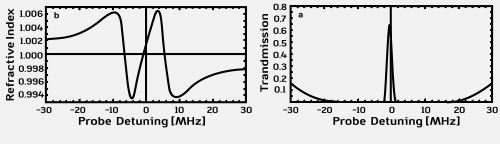
Figure 12: Refractive index variation with the frequency of a probe laser pulse.
Source: © Reprinted by permission from Macmillan Publishers Ltd: Nature 397, 594-598 (18 February 1999).
The refractive index and transmission are shown as functions of the frequency of the probe laser. A “detuning” of 0 MHz means that the probe laser frequency matches the energy difference between levels 1 and 3. The very rapid variation of the refractive index around 0 MHz created in this system is responsible for ultra-slow light. (Unit: 7)
Another interesting thing happens. In the absence of the coupling laser beam, the “probe” laser pulse would be completely absorbed because the probe laser is tuned to the energy difference between states 1 and 3, and the atoms start out in state 1 as we discussed above. When the atoms absorb probe photons, they jump from state 1 to state 3; after a brief time, the excited atoms relax by reemitting light, but at random and in all directions. The cloud would glow bright yellow, but all information about the original light pulse would be obliterated. Since we instead first turn the coupling laser on and then send the probe laser pulse in, this absorption is prevented. The two laser beams shift the atoms into a quantum superposition of states 1 and 2, meaning that each atom is in both states at once. State 1 alone would absorb the probe light, and state 2 would absorb the coupling beam, each by moving atoms to state 3, which would then emit light at random. Together, however, the two processes cancel out, like evenly matched competitors in a tug of war—an effect called quantum interference.
The superposition state is called a dark state because the atoms in essence cannot see the laser beams (they remain “in the dark”). The atoms appear transparent to the probe beam because they cannot absorb it in the dark state, an effect called “electromagnetically induced transparency.” Which superposition is dark—what ratio of states 1 and 2 is needed—varies according to the ratio of light in the coupling and probe beams at each location—more precisely, to the ratio of the electric fields of the probe pulse and coupling laser beam. Once the system starts in a dark state (as it does in this case: 100 percent coupling beam and 100 percent state 1), it adjusts to remain dark even when the probe beam lights up. The quantum interference effect is also responsible for the rapid variation of the refractive index that leads to slow light. The light speed can be controlled by simply controlling the coupling laser intensity: the lower the intensity, the steeper the slope, and the lower the light speed. In short, the light speed scales directly with the coupling intensity.
6. Implementing These Ideas in the Laboratory

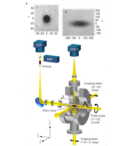
Figure 13: Experimental realization of slow light.
Source: © Reprinted by permission from Macmillan Publishers Ltd: Nature 397, 594-598 (18 February 1999).
The cigar-shaped, nanokelvin-cold atom cloud is held by the electromagnet in the middle of the vacuum chamber. The cloud is first illuminated from the side by the coupling laser beam, and then a probe laser pulse is injected. We wait behind the vacuum chamber for the light pulse to come out and measure the arrival time with a photomultiplier (PMT). To figure out the light’s speed, we also need to know how long the atom cloud is. We send a third laser beam (imaging beam) up through the cloud and the atoms create an absorption shadow in the beam that is imaged onto a camera. We now take a snapshot of the atom cloud that is seen at the top right of the figure. The atom cloud in this case is 229 micrometers long. (Unit: 7)
Figure 13 shows a typical setup that we actually use for slowing light. We hold the atom cloud fixed in the middle of the vacuum chamber with use of the electromagnet and first illuminate the atom cloud from the side with the coupling laser. Then we send the probe light pulse into the cooled atoms. We can make a very direct measurement of the light speed: We simply sit and wait behind the vacuum chamber for the light pulse to come out, and measure the arrival time of the light pulse. To figure out the light speed, we just need to know the length of the cloud. For this purpose, we send a third “imaging” laser beam into the chamber from down below, after the probe pulse has propagated through the atom cloud and the coupling laser is turned off.

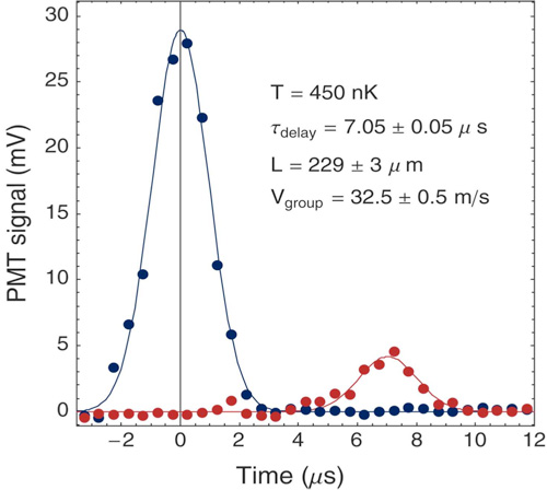
Figure 14: Measurement of ultra-slow light in a cold atom cloud.
Source: © Reprinted by permission from Macmillan Publishers Ltd: Nature 397, 594-598 (18 February 1999).
A probe light pulse propagates through the cold atom cloud shown in Figure 13 (Section 6) and is then measured with a photomultiplier. The data are recorded with an oscilloscope, and the result is the red pulse shown in the figure. The blue pulse is recorded with no atoms in the system and simply sets the zero point for the time axis. Since the light pulse takes 7 microseconds to travel though an atom cloud that is only 229 micrometers long, we can immediately conclude that light has been slowed to only 32 meters/second—slowed by a factor of 10 million! (Unit: 7)
As the imaging laser is tuned on resonance with the atom’s characteristic frequency, and there is only one laser beam present (i.e., there is no quantum interference), the atoms will absorb photons and create an absorption shadow in the imaging beam. By taking a photograph of this shadow with a camera, we can measure the length of the cloud. An example is seen in Figure 13 where the shadow (and the cloud) has a length of 0.008 inches. By sending a light pulse through precisely this cloud, we record the red light pulse in Figure 14. It takes the pulse 7 microseconds (7 millionths of a second) to get through the cloud. We now simply divide the cloud length by the propagation time to obtain the light speed of the light pulse: 71 miles/hour. So, we have already slowed light by a factor of 10 million. We can lower the intensity of the coupling beam further and propagate the pulse through a basically pure Bose-Einstein condensate to get to even lower light speeds of 15 miles/hour. At this point, you can easily beat light on your bicycle.
Figure 15 illustrates how the light pulse slows in the atom cloud: associated with the slowdown is a huge spatial compression of the light pulse. Before we send the pulse into the atom cloud, it has a length of roughly a mile [its duration is typically a few microseconds, and by multiplying the duration by the light speed in free space (186,000 miles per second), we get the length]. As the light pulse enters the cloud, the front edge slows down; but the back edge is still in free space, so that end will be running at the normal light speed. Hence, it will catch up to the front edge and the pulse will start to compress. The pulse is compressed by the same factor as it is slowed, so in the end, it is less than 0.001″ long, or less than half the thickness of a hair. Even though our atom clouds are small, the pulse ends up being even smaller, small enough to fit inside an atom cloud. The light pulse also makes an imprint in the atom cloud, really a little holographic imprint. Within the localized pulse region, the atoms are in these dark states we discussed earlier. The spatial modulation of the dark state mimics the shape of the light pulse: in the middle of the pulse where the electric field of the probe laser is high, a large fraction of an atom’s state is transferred from 1 to 2. At the fringe of the pulse, only a small fraction is in 2; and outside the light pulse, an atom is entirely in the initial state 1. The imprint follows the light pulse as it slowly propagates through the cloud. Eventually, the light pulse reaches the end of the cloud and exits into free space where the front edge takes off as the pulse accelerates back up to its normal light speed. In the process, the light pulse stretches out and regains the length it had before it entered the medium.
It is interesting to note that when the light pulse has slowed down, only a small amount of the original energy remains in the light pulse. Some of the missing energy is stored in the atoms to form the holographic imprint, and most is sent out into the coupling laser field. (The coupling photons already there stimulate new photons to join and generate light with the same wavelength, direction, and phase). When the pulse leaves the medium, the energy is sucked back out of the atoms and the coupling beam, and it is put back into the probe pulse.

Figure 15: Light slows down in a Bose-Einstein condensate.
Source: © Chien Liu and Lene V. Hau. A light pulse slows and, at the same time, spatially compresses in a Bose-Einstein condensate. As a matter of fact, the pulse compresses by the same factor as it slows down. The light pulse also creates a holographic imprint in the condensate, and that little imprint follows along as the pulse slowly propagates through the atom cloud. When the light pulse exits the condensate, it accelerates back up and stretches out again to regain the length it had before it entered the atom cloud.
Try to run the animation again and click on the screen when the pulse is slowed down, compressed, and contained in the atom cloud: The light pulse stops. You might ask: Could we do the same in the lab? The answer is: Yes, indeed, and it is just as easy—just block the coupling laser. As mentioned earlier, when the coupling intensity decreases, the light speed also decreases, and the light pulse comes to a halt. The atoms try to maintain the dark state. If the coupling laser turns off, the atoms will try to absorb probe light and emit some coupling light, but the light pulse runs empty before anything really changes. So, the light pulse turns off but the information that was in the pulse is not lost: it is preserved in the holographic imprint that was formed and that stays in the atom cloud.
Before we move on, it is interesting to pause for a moment. The slowing of light to bicycle speed in a Bose-Einstein condensate in 1999 stimulated a great many groups to push for achieving slow light. In some cases, it also stopped light in all kinds of media, such as hot gases, cooled solids, room temperature solids, optical fibers, integrated resonators, photonic crystals, and quantum wells, and with classical or quantum states of light. The groups include those of Scully at Texas A&M, Budker at Berkeley, Lukin and Walsworth at Harvard and CFA, Hemmer at Hanscom AFB, Boyd at Rochester, Chuang at UIUC, Chang-Hasnain at Berkeley, Kimble at Caltech (2004), Kuzmich at Georgia Tech, Longdell et al. in Canberra, Lipson at Cornell, Gauthier at Duke, Gaeta at Cornell, Vuckovic at Stanford, Howell at Rochester, and Mørk in Copenhagen, to name just a few.
7. Converting Light to Matter and Back: Carrying Around Light Pulses

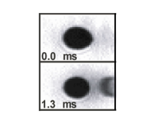
Figure 16: Turning light into matter with the creation of a perfect matter copy of the extinguished light pulse.
Source: © Reprinted by permission from Macmillan Publishers Ltd: Nature 445, 623-626 (8 February 2007).
The light pulse is first slowed, compressed, and extinguished in a Bose-Einstein condensate. The holographic imprint that the slowing light pulse created in the condensate starts to travel out of the atom cloud and into free space. After 1.3 milliseconds we have a perfect matter copy of the extinguished light pulse isolated in free space…and we photograph it. The atoms in the traveling matter copy are actually both traveling out in free space and stuck back in the condensate at the same time—remember, this is quantum mechanics. (Unit: 7)
Light and other electromagnetic waves carry energy, and that energy comes in quanta called “photons.” The energy of a photon is proportional to the frequency of the light with a constant of proportionality called Planck’s constant. We have already encountered photons on several occasions and seen that photons carry more than energy—they also carry momentum: an atom gets that little kick each time it absorbs or emits a photon.
When we slow, compress, stop, or extinguish a light pulse in a Bose-Einstein condensate, we end up with the holographic, dark state imprint where atoms are in states 1 and 2 at the same time. That part of an atom which is in state 2 got there by the absorption of a probe laser photon and the emission of a coupling laser photon. It has thus received two momentum kicks: one from each laser field. Therefore, the state 2 imprint starts to move slowly—at a few hundred feet per hour. It will eventually exit the condensate and move into free space.

Figure 17: The matter copy continues the journey.
Source: © Reprinted by permission from Macmillan Publishers Ltd: Nature 445, 623-626 (8 February 2007).
After creation of a perfect matter copy of a light pulse that was extinguished in the first Bose-Einstein condensate (left), the matter copy travels in free space to a second Bose-Einstein condensate (right). If we don’t do anything, the matter copy simply travels through this second condensate and exits on the other side. (Unit: 7)
At this point, we have created, out in free space, a matter copy of the light pulse that was extinguished. This matter copy can be photographed as shown in Figure 16. It takes the matter copy roughly one-half millisecond to exit the condensate, and we note that it has a boomerang shape. Why? Because when the light pulse slows down in the condensate, it slows most along the centerline of the condensate where the density of atoms is highest. Therefore, the light pulse itself develops a boomerang shape, which is clearly reflected in its flying imprint.
It is also interesting to remember that the atoms are in a superposition of quantum states: An atom in the matter copy is actually both in the matter copy traveling along and at the same time stuck back in the original condensate. When we photograph the matter copy, however, we force the atoms to make a decision as to “Am I here, or am I there?” The wavefunction collapses, and the atom is forced into a single definite quantum state. If we indeed have at hand a perfect matter copy of the light pulse, it should carry exactly the same information as the light pulse did before extinction; so could we possibly turn the matter copy back into light? Yes.

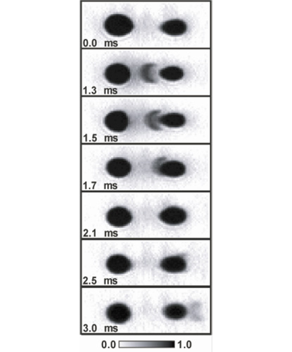
Figure 18: Turning light into matter in one BEC and then matter back into light in a second BEC in a different location.
Source: © Reprinted by permission from Macmillan Publishers Ltd: Nature 445, 623-626 (8 February 2007).
When the matter copy is embedded in the second Bose-Einstein condensate we simply illuminate with the coupling laser, and the light pulse is regenerated from the second condensate. This happens even though the light pulse was extinguished in a totally different condensate at a different location. Altogether, we have stopped and extinguished a light pulse in one location, turned it into a matter copy, carried it over to another location, and turned the matter copy back to light. (Unit: 7)
To test this, we form a whole different condensate of atoms in a different location, and we let the matter copy move into this second condensate. Two such condensates are shown in Figure 17. In these experiments, the light pulse comes in from the left and is stopped and extinguished in the first (leftmost) condensate. The generated matter copy travels into and across free space, and at some point it reaches the second (rightmost) condensate. If we don’t do anything, the matter copy will just go through the condensate and come out on the other side at 2.5 ms and 3.0 ms (See Figure 18). On the other hand, once the matter copy is imbedded in the second condensate, if we turn on the coupling laser…out comes the light pulse! The regenerated light pulse is shown in Figure 18a.
So here, we have stopped and extinguished a light pulse in one condensate and revived it from a completely different condensate in a different location. Try to run the animation in Figure 19 and test this process for yourself.

Figure 19: A light pulse is extinguished in one part of space and then regenerated in a different location.
Source: © Sean Garner and Lene V. Hau.
The orange coupling laser first illuminates a Bose-Einstein condensate from the right. A yellow input light pulse is injected from the left into the first condensate where it is slowed and then extinguished. A perfect matter copy (red) of the light pulse is created, and this messenger atom pulse travels across to the second condensate where the matter copy is converted back to light.
Quantum puzzles
The more you think about this, the weirder it is. This is quantum mechanics seriously at play. The matter copy and the second receiver condensate consist of two sets of atoms that have never seen each other, so how can they together figure out to revive the light pulse? The secret is that we are dealing with Bose-Einstein condensates. When we illuminate the atoms in the matter copy with the coupling laser, they act as little radiating antennae. Under normal circumstances, these antennae would each do its own thing, and the emitted radiation would be completely random and contain no information. However, the lock-step nature of the receiver condensate will phase lock the antennae so they all act in unison, and together they regenerate the light pulse with its information preserved. When the light pulse is regenerated, the matter copy atoms are converted to state 1 and added as a bump on the receiver condensate at the revival location. The light pulse slowly leaves the region, exits the condensate, and speeds up.
This demonstrated ability to carry around light pulses in matter has many implications. When we have the matter copy isolated in free space, we can grab onto it—for example, with a laser beam—and put it “on the shelf” for a while. We can then bring it to a receiver condensate and convert it back into light. And while we are holding onto the matter copy, we can manipulate it, change its shape—its information content. Whatever changes we make to the matter copy will then be contained in the revived light pulse. In Figure 18b, you see an example of this: During the hold time, the pulse is changed from a single-hump to a double-hump pulse.
You might ask: How long can we hold on to a light pulse? The record so far is a few seconds. During this time, light can go from the Earth to the Moon! In these latest experiments, we let the probe and coupling beams propagate in the same direction; so there is basically no momentum kick to the matter imprint, and it stays in the atom condensate where it was created. When atoms in the matter imprint collide with the host condensate, they can scatter to states other than 1 and 2. This will lead to loss of atoms from the imprint and therefore to loss of information. By exposing the atom cloud to a magnetic field of just the right magnitude, we can minimize such undesired interactions between the matter imprint and the host condensate. Even more, we can bring the system into a phase-separating regime where the matter imprint wants to separate itself from the host condensate, much like an oil drop in water. The matter imprint digs a hole for itself in the host, and the imprint can snugly nestle there for extended time scales without suffering damaging collisions. Also, we can move the matter imprint to the opposite tip of the condensate from where it came in, and the imprint can now be converted to light that can immediately exit the condensate without losses. This shows some of the possibilities we have for manipulating light pulses in matter form.
8. Potential Long-Term Applications: Quantum Processing
The best and most efficient way to transport information is to encode it in light and send it down an optical fiber where it can propagate with low loss and at high data rates. This process is used for information traveling over the Internet. However to manipulate—or process—the information, it is much better to have it in matter form, as you can grab matter and easily change it. In current fiber optical networks, optical pulses are changed to electronic signals at nodes in the network. However, in these systems with existing conversion methods, the full information capacity of light pulses cannot be utilized and maintained. Using instead the methods described above, all information encoded in light—including its quantum character—can be preserved during conversion between light and matter, and the information can be powerfully processed. This is particularly important for creating quantum mechanical analogues of the Internet. Transport and processing of data encoded in quantum states can be used for teleportation and secure encryption. The ability to process quantum information is needed for the development of quantum computers.

Figure 20: Classical computers use bits that can be valued either 0 or 1.
In a classical computer numbers are represented by strings of bits that can each have only two values: 0 or 1. For example, the number 5 written in binary form is represented by the bit string 101. The result of a calculation performed with a classical computer is stored in an output register as a string of 0s and 1s. (Unit: 7)
One possible application of the powerful methods for light manipulation described above is in quantum computing. In our current generation of computers, data are stored in memory as bit patterns of 0s and 1s (binary numbers). In a quantum computer, the 1s and 0s are replaced with quantum superpositions of 1s and 0s, called qubits, which can be 0 and 1 at the same time. Such computers, if they can be built, can solve a certain set of hard problems that it would take an ordinary computer a very long time (longer than the life of the universe) to crack. The trick is that because of quantum superposition, the input bit register in a quantum computer can hold all possible input values simultaneously, and the computer can carry out a large number of calculations in parallel, storing the results in a single output register. Here we get to another important aspect of quantum computing:entanglement.
Let’s look at a simple case of entanglement, involving a light pulse containing a single photon (i.e., we have a single energy quantum in the light pulse. There is some discussion as to whether this is a case of true entanglement, but it serves to illustrate the phenomenon in any case). If we send the photon onto a beamsplitter, it has to make a choice between two paths. Or rather, quantum mechanics allows the photon to not actually make up its mind: The photon takes both paths at the same time. We can see this through interference patterns that are made even when the photon rate is so low that less than one photon is traveling at a time. But if we set up a light detector to monitor one of the two paths, we will register a click (a photon hit) or no click, each with a 50% chance. Now say some other (possibly distant) observer sets up a detector to monitor the other path. In this case, if this second observer detects a click, that instantaneously affects our own measurement: We will detect “no click” with 100% probability (or vice versa, an absolutely certain click if the remote observer has detected no click), since each photon can be detected only once. And this happens even in cases where the detectors are at a very large distance from each other. This is entanglement: the quantum correlation of two spatially separated quantum states. The fact that a measurement in one location on part of an entangled state immediately affects the other part of the state in a different location—even if the two locations are separated by a very large distance—is a nonlocal aspect of quantum mechanics. Entangled states are hard to maintain, because interactions with the environment destroy the entanglement. They thus rarely appear in our macroscopic world, but that doesn’t stop them from being essential in the quantum world.

Figure 21: Quantum computers use qubits.
In a quantum computer, bits are replaced by qubits. Input and output registers consist of a number of qubits. These qubits do not have to be either 0 or 1. Rather, they can be in superposition states: 0 and 1 at the same time. (Unit: 7)
Now that we know what entanglement is, let’s get back to the quantum computer. Let’s say the quantum computer is set up to perform a particular calculation. One example would be to have the result presented at the output vary periodically with the input value (for example, if the computer calculates the value of the sine function). We wish to find the repetition period. The input and output registers of the computer each consist of a number of quantum bits, and the quantum computation leaves these registers in a superposition of matched pairs, where each pair has the output register holding the function value for the corresponding input register value. This is, in fact, an entangled state of the two registers, and the entanglement allows us to take advantage of the parallelism of the quantum computation. As in the beamsplitter example described above, a measurement on the output register will immediately affect the input register that will be left holding the value that corresponds to the measured output value. If the output repeats periodically as we vary the input, many inputs will correspond to a particular output, and the input register ends up in a superposition of precisely these inputs. This represents a great advantage over a classical calculation: After just one run-through of the calculation, global information—the repetition period—is contained in the input register. After a little “fiddling,” this period can be found and read back out with many fewer operations than a classical computer requires. In a classical calculation, we would have to run the computation many times—one for each input value—to slowly, step by step, build up information about the periodicity.

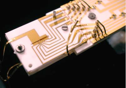
Figure 22: A two-bit quantum computer implemented with two beryllium ions trapped in a slit in an alumina substrate with gold electrodes.
Source: © J. Jost, NIST.
Two beryllium ions, each acting as a quantum bit, are trapped inside a 3.5 mm by 200 micrometer slit in an alumina wafer with gold electrodes. The slit is seen as a narrow dark slit on the left side of the chip. This chip-based quantum computer was produced by David Wineland’s group at the National Institute of Standards and Technology (NIST), Colorado. Wineland’s team can perform a controlled sequence of 25 one and two-bit operations with the system. (Unit: 7)
Whether quantum computers can be turned into practical devices remains to be seen. Some of the questions are: Can the technology be scaled? That is, can we generate systems with enough quantum bits to be interesting? Is the processing (the controlled change of quantum states) fast enough that it happens before coupling to the surroundings leads to “dephasing,” that is to destruction of the superposition states and the entanglement? Many important experiments aimed at the implementation of a quantum computer have been performed, and quantum computing with a few qubits has been successfully carried out, for example, with ions trapped in magnetic traps (See Figure 22). Here, each ion represents a quantum bit, and two internal states of the ion hold the superposition state corresponding to the quantum value of the bit. Encoding quantum bits—or more generally quantum states—via slow light-generated imprints in Bose-Einstein condensates presents a new and interesting avenue toward implementation of quantum computation schemes: The interactions between atoms can be strong, and processing can happen fast. At the same time, quantum dephasing mechanisms can be minimized (as seen in the experiments with storage times of seconds). Many light pulses can be sent into a Bose-Einstein condensate and the generated matter copies can be stored, individually manipulated, and led to interact. One matter copy thus gets affected by the presence of another, and these kinds of operations—called conditional operations—are of major importance as building blocks for quantum computers where generation of entanglement is essential. After a series of operations, the resulting quantum states can be read back out to the optical field and communicated over long distances in optical fibers.

Figure 23: A Bose-Einstein condensate as a novel processor for quantum information.
Source: © Zachary Dutton and Lene V. Hau.
Another potential application of slow light-based schemes for quantum information processing, which has the promise to be of more immediate, practical use, is for secure encryption of data sent over a communication network (for example, for protecting your personal information when you send it over the Internet). Entangled quantum states can be used to generate secure encryption keys. As described above with the photon example, two distant observers can each make measurements on an entangled state. If we make a measurement we will immediately know what the other observer will measure. By generating and sharing several such entangled quantum states, a secure encryption key can be created. The special thing with quantum states is that if a spy listens in during transmission of the key, we would know: If a measurement is performed on a quantum state, it changes—once again: The wavefunction “collapses.” So the two parties can use some of the shared quantum states as tests: They can communicate the result of their measurements using their cell phones. If there is not a complete agreement between expected and actual measurements at the two ends, it is a clear indication that somebody is listening in and the encryption key should not be used.
An efficient way to generate and transport entangled states can be achieved with the use of light (as in our photon example above) transmitted in optical fibers. However, the loss in fibers is not negligible, and entanglement distribution over long distances (above 100 km, say) has to be made in segments. Once the individual segments are entangled, they must then be connected in pairs to distribute the entanglement between more distant locations. For this to be possible, we must be able to sustain the entanglement achieved in individual segments such that all the segments can eventually be connected. And here, the achievement of hold times for light of several seconds, as described above, is really important.

Figure 24: Was Newton right after all: “Are not gross Bodies and Light convertible into one another… ?”
Light to matter and back to light—made possible with slow light in Bose-Einstein condensates. (Unit: 7)
There are numerous applications for slow and stopped light, and we have explored just a few of them here. The important message is that we have achieved a complete symmetry between light and matter, and we get there by making use of both lasers and Bose-Einstein condensates. A light pulse is converted to matter form, and the created matter copy—a perfect imitation of the light pulse that is extinguished—can be manipulated: put on the shelf, moved, squeezed, and brought to interact with other matter. At the end of the process, we turn the matter copy back into light and beam it off at 186,000 miles per hour. During formation of the matter copy—by the slowing and imprinting of the input light pulse in a Bose-Einstein condensate—it is essential that the coupling laser field is present with its many photons that are all in lock-step. And when the manipulated matter copy is transformed back into light, the presence of many atoms in the receiver (or host) BEC that are all in lock-step is of the essence.
So, we have now come full circle: From Newton over Huygens, Young, and Maxwell, we are now back to Newton:
In Opticks, published in 1704, Newton theorized that light was made of subtle corpuscles and ordinary matter of grosser corpuscles. He speculated that through an alchemical transmutation, “Are not gross Bodies and Light convertible into one another, …and may not Bodies receive much of their Activity from the Particles of Light which enter their Composition?”
9. Further Reading
- Video lectures on quantum computing by Oxford Professor David Deutsch: http://www.quiprocone.org/Protected/DD_lectures.htm.
- Lene Vestergaard Hau,”Frozen Light,” Scientific American, 285, 52-59 (July 2001), and Special Scientific American Issue entitled, “The Edge of Physics” (2003).
- Lene Vestergaard Hau, “Taming Light with Cold Atoms,” Physics World 14, 35-40 (September 2001). Invited feature article. Published by Institute for Physics, UK.
- Simon Singh, “The Code Book: The Science of Secrecy from Ancient Egypt to Quantum Cryptography,” Anchor, reprint edition (August 29, 2000).