


Physics for the 21st Century
String Theory and Extra Dimensions Online Textbook
Online Text by Shamit Kachru
The videos and online textbook units can be used independently. When using both, it is possible to start with either one. Watching the video first, and then reading the unit from the online textbook is recommended.
Each unit was written by a prominent physicist who describes the cutting edge advances in his or her area of research and the potential impacts of those advances on everyday life. The classical physics related to each new topic is covered briefly to help the reader better understand the research, its effects, and our current understanding of physics.
Click on “Content By Unit” (in the menu to the left) and select a unit title to view the Web version of the online text, which includes links to related material. Or, download PDF versions of the units below.
1. Introduction
The first two units of this course have introduced us to the four basic forces in nature and the efforts to unify them in a single theory. This quest has already been successful in the case of the electromagnetic and weak interactions, and we have promising hints of a further unification between the strong interactions and the electroweak theory (though this is far from experimentally tested). However, bringing gravity into this unified picture has proven far more challenging, and fundamental new theoretical issues come to the forefront. To reach the ultimate goal of a “theory of everything” that combines all four forces in a single theoretical framework, we first need a workable theory of quantum gravity.

Figure 1: The fundamental units of matter may be minuscule bits of string.
Source: © Matt DePies, University of Washington.
In the past century, physicists have discovered new constituents of matter—quarks, gluons, neutrinos, and many others. These basic building blocks have been linked together into a theoretical framework, the Standard Model of particle physics, that has been very successful in making predictions that were later confirmed by experiment. Even so, there are hints that the Standard Model is incomplete, and that a deeper theory lies behind it, waiting to be teased into the open. See how scientists are seeking answers to these questions with the latest neutrino experiments and the search for the Higgs boson.
As we saw in Units 2 and 3, theorists attempting to construct a quantum theory of gravity must somehow reconcile two fundamentals of physics that seem irreconcilable—Einstein’s general theory of relativity and quantum mechanics. Since the 1920s, that effort has produced a growing number of approaches to understanding quantum gravity. The most prominent at present is string theory—or, to be accurate, an increasing accumulation of string theories. Deriving originally from studies of the strong nuclear force, the string concept asserts that the fundamental units of matter are not the traditional point-like particles but miniscule stretches of threadlike entities called “strings.”
One of the most striking qualitative features of the string theories is that they predict the existence of extra spatial dimensions, with a total of 10 spacetime dimensions in the best-studied variants of the theory. This multitude of extra dimensions, beyond the familiar three of space plus one of time, suggests new approaches to account for some of the unsolved puzzles in the Standard Model of particle physics. String theory also has the potential to provide insights into the ultimate puzzles of cosmology, such as the nature of the Big Bang and the origin of dark matter and dark energy that we will learn more about in Units 10 and 11.

Figure 2: Above each point in our visible dimensions, a small extra-dimensional space may be hidden.
Source: © BCCP, Lawrence Berkeley National Laboratory.
However, candidates for an acceptable framework that combines gravity with the other three fundamental forces have one characteristic that separates them, and this unit, from all of the other topics covered in this course: Quantum gravity theories in general, and string theories in particular, have virtually no connection (as yet) to experimental evidence. There is, so far, no evidence that string theory is the correct modification of Einstein’s theory, which would render it compatible with quantum mechanics in our world. String theories, or at least most models that follow from string theory, are only predictive at energy scales far from what can be probed with current particle physics and cosmological observations. This is not surprising; it follows from basic dimensional analysis, which we will describe in this unit, and which suggests that we will need a great deal of luck (or a very big accelerator) to directly test any approach to quantum gravity. Enthusiasm for string theory has been based, instead, on the theoretical richness and consistency of the structure it gives rise to, as well as the fruitful connections it has enjoyed with many other areas of physics. But one should keep in mind that its proponents will eventually need to make experimental predictions that can be tested to confirm or deny the validity of the approach as a literal description of quantum gravity in our universe.
In the following sections, we will see some current frontiers of physics where the quantum properties of gravity may be visible in near-term experiments studying the interactions of elementary particles at very high energy, or the physics of the very early universe. We hope, then, to gain one or more experimental windows (albeit very indirect ones) into the world of quantum gravity.
2. The Origins of Quantum Gravity
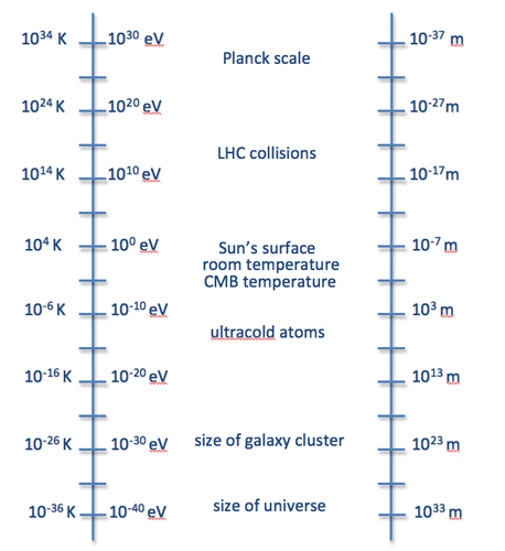
In the early 20th century, physicists succeeded in explaining a wide range of phenomena on length scales ranging from the size of an atom (roughly 10-8 centimeters) to the size of the currently visible universe (roughly 1028 centimeters). They accomplished this by using two different frameworks for physical law: quantum mechanics and the general theory of relativity.

The length scale shown above is logarithmic, and each tick mark represents a distance 100,000 times longer than the one below it. This span of lengths, from roughly 1030 m on the large end to 10-35 m on the small end, covers all of physics as we know it. It’s not possible for something to be larger than the size of the universe, and we’re not sure that it even makes sense to talk about a length smaller than the Planck length. We know that general relativity dominates at large scales, where we find galaxy clusters and mountains, and that quantum mechanics dominates at small scales, where we find molecules, atoms, and possibly even strings. The two theories meet somewhere in the middle of the scale, where a theory of quantum gravity is essential. Note that the short-distance tests of gravity described in Unit 3 take place right in the center of the scale, at around 10-4 m. (Unit: 4)
Built on Albert Einstein’s use of Max Planck’s postulate that light comes in discrete packets called “photons” to explain the photoelectric effect and Niels Bohr’s application of similar quantum ideas to explain why atoms remain stable, quantum mechanics quickly gained a firm mathematical footing. (“Quickly” in this context, means over a period of 25 years). Its early successes dealt with systems in which a few elementary particles interacted with each other over short distance scales, of an order the size of an atom. The quantum rules were first developed to explain the mysterious behavior of matter at those distances. The end result of the quantum revolution was the realization that in the quantum world—as opposed to a classical world in which individual particles follow definite classical trajectories—positions, momenta, and other attributes of particles are controlled by a wave function that gives probabilities for different classical behaviors to occur. In daily life, the probabilities strongly reflect the classical behavior we intuitively expect; but at the tiny distances of atomic physics, the quantum rules can behave in surprising and counterintuitive ways. These are described in detail in Units 5 and 6.
In roughly the same time period, but for completely different reasons, an equally profound shift in our understanding of classical gravity occurred. One of the protagonists was again Einstein, who realized that Newton’s theory of gravity was incompatible with his special theory of relativity. In Newton’s theory, the attractive gravitational force between two bodies involves action at a distance. The two bodies attract each other instantaneously, without any time delay that depends on their distance from one another. The special theory of relativity, by contrast, would require a time lapse of at least the travel time of light between the two bodies. This and similar considerations led Einstein to unify Newtonian gravity with special relativity in his general relativity theory.
Einstein proposed his theory in 1915. Shortly afterward, in the late 1920s and early 1930s, theorists found that one of the simplest solutions of Einstein’s theory, called the Friedmann-Lemaître-Robertson-Walker cosmology after the people who worked out the solution, can accommodate the basic cosmological data that characterize our visible universe. As we will see in Unit 11, this is an approximately flat or Euclidean geometry, with distant galaxies receding at a rate that gives us the expansion rate of the universe. This indicates that Einstein’s theory seems to hold sway at distance scales of up to 1028 centimeters.
In the years following the discoveries of quantum mechanics and special relativity, theorists worked hard to put the laws of electrodynamics and other known forces (eventually including the strong and weak nuclear forces) into a fully quantum mechanical framework. The quantum field theory they developed describes, in quantum language, the interactions of fields that we learned about in Unit 2.
The theoretical problem of quantizing gravity
In a complete and coherent theory of physics, one would like to place gravity into a quantum framework. This is not motivated by practical necessity. After all, gravity is vastly weaker than the other forces when it acts between two elementary objects. It plays a significant role in our view of the macroscopic world only because all objects have positive mass, while most objects consist of both positive and negative electric charges, and so become electromagnetically neutral. Thus, the aggregate mass of a large body like the Earth becomes quite noticeable, while its electromagnetic field plays only a small role in everyday life.

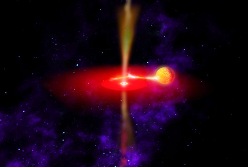
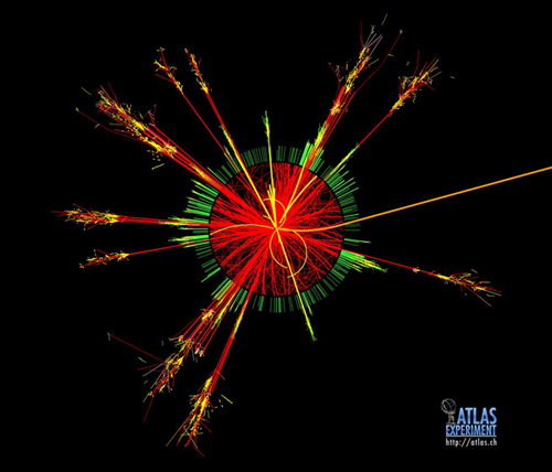
Figure 4: The rules of quantum gravity must predict the probability of different collision fragments forming at the LHC, such as the miniature black hole simulated here.
Source: © ATLAS Experiment, CERN.
Particle accelerators such as the LHC smash particles together at high energies, producing a wide variety of different collision fragments. Although the collision energies obtained in the LHC are far from the Planck scale, a good theory of quantum gravity must correctly predict the probability of different particles being produced in the collisions. The image shown here is a simulated event in the ATLAS detector, in which a miniature black hole is produced and immediately decays into a multitude of other particles. (Unit: 4)
But while the problem of quantizing gravity has no obvious practical application, it is inescapable at the theoretical level. When we smash two particles together at some particular energy in an accelerator like the Large Hadron Collider (LHC), we should at the very least expect our theory to give us quantum mechanical probabilities for the nature of the resulting collision fragments.
Gravity has a fundamental length scale—the unique quantity with dimensions of length that one can make out of Planck’s constant, Newton’s universal gravitational constant, G, and the speed of light, c. The Planck length is 1.61 x 10⁻³⁵ meters, 1020 times smaller than the nucleus of an atom. A related constant is the Planck mass (which, of course, also determines an energy scale); is around 10-5 grams, which is equivalent to ~ 1019 giga-electron volts (GeV). These scales give an indication of when quantum gravity is important, and how big the quanta of quantum gravity might be. They also illustrate how in particle physics, energy, mass, and 1/length are often considered interchangeable, since we can convert between these units by simply multiplying by the right combination of fundamental constants. See The Math section below.
Since gravity has a built-in energy scale, MPlanck, we can ask what happens as we approach the Planckian energy for scattering. Simple approaches to quantum gravity predict that the probability of any given outcome when two energetic particles collide with each other grows with the energy, E, of the collision at a rate controlled by the dimensionless ratio (E/MPlanck)2. This presents a serious problem: At some energy close to the Planck scale, one finds that the sum of the probabilities for final states of the collision is greater than 100%. This contradiction means that brute-force approaches to quantizing gravity are failing at sufficiently high energy.
We should emphasize that this is not yet an experimentally measured problem. The highest energy accelerator in the world today, the LHC, is designed to achieve center-of-mass collision energies of roughly 10 tera-electron volts (TeV)—15 orders of magnitude below the energies at which we strongly suspect that quantum gravity presents a problem.

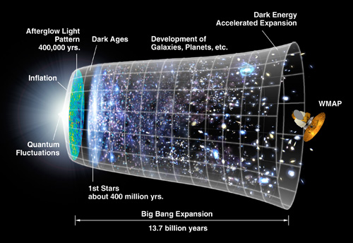
Figure 5: General relativity is consistent with all the cosmological data that characterizes our visible universe.
Source: © NASA, WMAP Science Team.
The diagram above outlines the history of our universe, from the Big Bang up to the present, taking into account many different types of cosmological observations. We have observed relic photons from the time atoms first formed, the distribution of galaxies and galaxy clusters that formed as overdense regions in the early universe collapsed, and the shift to the red in the spectra of distant supernovae that indicates that the universe is expanding. All of these observations, and many others, are consistently described by general relativity, which gives us confidence that Einstein’s theory holds true at distance scales up to 1028 cm. There is also strong evidence to support the period of rapid expansion (called “inflation”) on the left side of the diagram, which string theory may actually be able to explain. (Unit: 4) General relativity is consistent with all the cosmological data that characterizes our visible universe.
On the other hand, this does tell us that somewhere before we achieve collisions at this energy scale (or at distance scales comparable to 10-32 centimeters), the rules of gravitational physics will fundamentally change. And because gravity in Einstein’s general relativity is a theory of spacetime geometry, this also implies that our notions of classical geometry will undergo some fundamental shift. Such a shift in our understanding of spacetime geometry could help us resolve puzzles associated with early universe cosmology, such as the initial cosmological singularity that precedes the Big Bang in all cosmological solutions of general relativity.
These exciting prospects of novel gravitational phenomena have generated a great deal of activity among theoretical physicists, who have searched long and hard for consistent modifications of Einstein’s theory that avoid the catastrophic problems in high-energy scattering and that yield new geometrical principles at sufficiently short distances. As we will see, the best ideas about gravity at short distances also offer tantalizing hints about structures that may underlie the modern theory of elementary particles and Big Bang cosmology.
3. String Theory
Almost by accident in the mid 1970s, theorists realized that they could obtain a quantum gravity theory by postulating that the fundamental building blocks of nature are not point particles, a traditional notion that goes back at least as far as the ancient Greeks, but instead are tiny strands of string. These strings are not simply a smaller version of, say, our shoelaces. Rather, they are geometrical objects that represent a fundamentally different way of thinking about matter. This family of theories grew out of the physics of the strong interactions. In these theories, two quarks interacting strongly are connected by a stream of carriers of the strong force, which forms a “flux tube.” The potential energy between the two quarks, therefore, grows linearly with the distance between the quarks. See The Math section below.

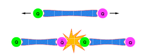
Figure 6: As quarks are pulled apart, eventually new quarks appear.
Source: © David Kaplan.
Quarks are bound together by the strong interaction. Bound quarks are constantly exchanging virtual gluons, which we can think of as forming a flux tube similar to a string stretching between the two particles. As the quarks are pulled apart, the potential energy between them grows, and is eventually equal to the amount of energy required to create two more quarks. At this point, the flux tube or string breaks, two more quarks are formed, and the quarks are once again bound in pairs. The string-like nature of the bond between quarks prompted theorists to think about what would happen if strings were fundamental quantum particles back in the 1960s. (Unit: 4)
We choose to call the proportionality constant that turns the distance between the strongly interacting particles into a quantity with the units of energy “Tstring” because it has the dimensions of mass per unit length as one would expect for a string’s tension. In fact, one can think of the object formed by the flux tube of strong force carriers being exchanged between the two quarks as being an effective string, with tension Tstring.
One of the mysteries of strong interactions is that the basic charged objects—the quarks—are never seen in isolation. The string picture explains this confinement: If one tries to pull the quarks farther and farther apart, the growing energy of the flux tube eventually favors the creation of another quark/anti-quark pair in the middle of the existing quark pair; the string breaks, and is replaced by two new flux tubes connecting the two new pairs of quarks. For this reason and others, string descriptions of the strong interactions became popular in the late 1960s. Eventually, as we saw in Unit 2, quantum chromodynamics (QCD) emerged as a more complete description of the strong force. However, along the way, physicists discovered some fascinating aspects of the theories obtained by treating the strings not as effective tubes of flux, but as fundamental quantum objects in their own right.
Perhaps the most striking observation was the fact that any theory in which the basic objects are strings will inevitably contain a particle with all the right properties to serve as a graviton, the basic force carrier of the gravitational force. While this is an unwanted nuisance in an attempt to describe strong interaction physics, it is a compelling hint that quantum string theories may be related to quantum gravity.

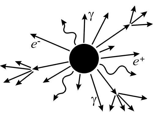
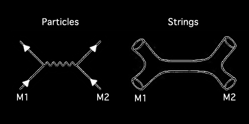
Figure 7: Gravitons arise naturally in string theory, leading to Feynman diagrams like the one on the right.
By analogy to the other three forces of nature, we assume that the gravitational interaction is mediated by a particle called the “graviton.” Gravitonal interactions in a traditional particle theory can be represented by Feynman diagrams like the one on the left, in which two massive particles, M1 and M2, interact by exchanging a graviton, represented by the squiggly line. The gravitational interaction changes the energy and momentum of M1 and M2. This graviton type of exchange emerges naturally from string theories, where the lowest mode of the string vibration gives rise to a set of particles that includes a graviton. We can represent the string theory version of graviton exchange with the diagram on the right, where point particles have been replaced by closed loops of string. In both diagrams, time increases in the vertical direction. (Unit: 4)
In 1984, Michael Green of Queen Mary, University of London and John Schwarz of the California Institute of Technology discovered the first fully consistent quantum string theories that were both free of catastrophic instabilities of the vacuum and capable in principle of incorporating the known fundamental forces. These theories automatically produce quantum gravity and force carriers for interactions that are qualitatively (and in some special cases even quantitatively) similar to the forces like electromagnetism and the strong and weak nuclear forces. However, this line of research had one unexpected consequence: These theories are most naturally formulated in a 10-dimensional spacetime.
We will come back to the challenges and opportunities offered by a theory of extra spacetime dimensions in later sections. For now, however, let us examine how and why a theory based on strings instead of point particles can help with the problems of quantum gravity. We will start by explaining how strings resolve the problems of Einstein’s theory with high-energy scattering. In the next section, we discuss how strings modify our notions of geometry at short distances.
Strings at high energy
In the previous section, we learned that for particles colliding at very high energies, the sum of the probabilities for all the possible outcomes of the collision calculated using the techniques of Unit 2 is greater than 100 percent, which is clearly impossible. Remarkably, introducing an extended object whose fundamental length scale is not so different from the Planck length,  ~ 10-32 centimeters, seems to solve this basic problem in quantum gravity. The essential point is that in high-energy scattering processes, the size of a string grows with its energy.

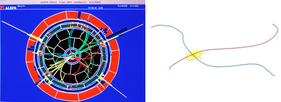
Figure 8: String collisions are softer than particle collisions.
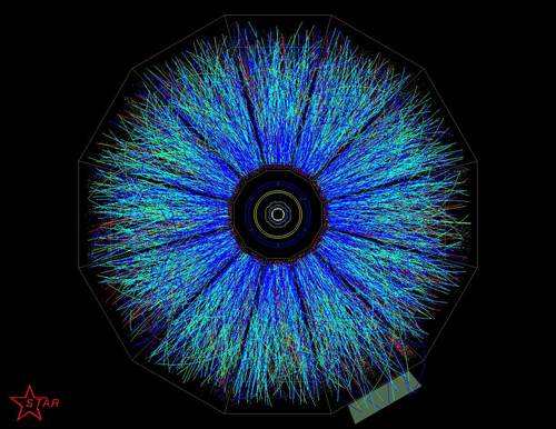
Source: © Left: CERN, Right: Claire Cramer.
In the collision shown on the left, electrons and positrons collide head-on in the ALEPH detector at CERN, producing a shower of other particles. The electrons and positrons are point particles, and the collision energy is the sum of the energies of the particles that hit one another. The collision of two strings sketched on the right is fundamentally different because the size of a string grows with its energy. A highly energetic string will be very long. When two energetic strings collide, the collision will only involve a small portion of each string, so the string collision is softer than the point particle collision. (Unit: 4)
This growth-with-energy of an excited string state has an obvious consequence: When two highly energetic strings interact, they are both in the form of highly extended objects. Any typical collision involves some small segment of one of the strings exchanging a tiny fraction of its total energy with a small segment of the other string. This considerably softens the interaction compared with what would happen if two bullets carrying the same energy undergo a direct collision. In fact, it is enough to make the scattering probabilities consistent with the conservation of probability. In principle, therefore, string theories can give rise to quantum mechanically consistent scattering, even at very high energies.
4. Strings and Extra Dimensions

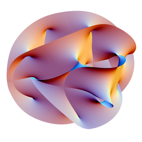
Figure 9: A depiction of one of the six-dimensional spaces that seem promising for string compactification.
Source: © Wikimedia Commons, CC Attribution-Share Alike 2.5 Generic license. Author: Lunch, 23 September 2007.
The string theories that correspond to quantum gravity, combined with the three other known forces, seem to require ten spacetime dimensions. We clearly live in four spacetime dimensions, so it is generally assumed that the other six dimensions must be curled up, or compactified, in a way that makes them impossible for us to see directly. The geometry of these compactified dimensions is complicated and difficult to visualize. The above image is a two-dimensional projection of a six-dimensional space that the compactified extra dimensions of string theory could occupy. (Unit: 4)
We have already mentioned that string theories that correspond to quantum gravity together with the three other known fundamental forces seem to require 10 spacetime dimensions. While this may come as a bit of a shock—after all, we certainly seem to live in four spacetime dimensions—it does not immediately contradict the ability of string theory to describe our universe. The reason is that what we call a “physical theory” is a set of equations that is dictated by the fundamental fields and their interactions. Most physical theories have a unique basic set of fields and interactions, but the equations may have many different solutions. For instance, Einstein’s theory of general relativity has many nonphysical solutions in addition to the cosmological solutions that look like our own universe. We know that there are solutions of string theory in which the 10 dimensions take the form of four macroscopic spacetime dimensions and six dimensions curled up in such a way as to be almost invisible. The hope is that one of these is relevant to physics in our world.
To begin to understand the physical consequences of tiny, curled-up extra dimensions, let us consider the simplest relevant example. The simplest possibility is to consider strings propagating in nine-dimensional flat spacetime, with the 10th dimension curled up on a circle of size R. This is clearly not a realistic theory of quantum gravity, but it offers us a tantalizing glimpse into one of the great theoretical questions about gravity: How will a consistent theory of quantum gravity alter our notions of spacetime geometry at short distances? In string theory, the concept of curling up, or compactification, on a circle, is already startlingly different from what it would be in point particle theory.

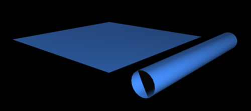
Figure 10: String theorists generally believe that extra dimensions are compactified, or curled up.
String theorists generally believe that extra dimensions are compactified, or curled up, so that the ten-dimensional spacetime required for string theory to combine gravity with the other forces of nature appears to be four-dimensional. A simple example of compactification leading to an apparently smaller number of dimensions is a flat sheet rolled into a tube. The flat sheet is two-dimensional, but when rolled into a cylinder with a very small radius, appears to be a one-dimensional line. (Unit: 4)
To compare string theory with normal particle theories, we will compute the simplest physical observable in each kind of theory, when it is compactified on a circle from ten to nine dimensions. This simplest observable is just the masses of elementary particles in the lower-dimensional space. It will turn out that a single type of particle (or string) in 10 dimensions gives rise to a whole infinite tower of particles in nine dimensions. But the infinite towers in the string and particle cases have an important difference that highlights the way that strings “see” a different geometry than point particles.
Particles in a curled-up dimension
Let us start by explaining how an infinite tower of nine-dimensional (9D) particles arises in the 10-dimensional (10D) particle theory. To a 9D observer, the velocity and momentum of a given particle in the hidden tenth dimension, which is too small to observe, are invisible. But the motion is real, and a particle moving in the tenth dimension has a nonzero energy. Since the particle is not moving around in the visible dimensions, one cannot attribute its energy to energy of motion, so the 9D observer attributes this energy to the particle’s mass. Therefore, for a given particle species in the fundamental 10D theory, each type of motion it is allowed to perform along the extra circle gives rise to a new elementary particle from the 9D perspective.

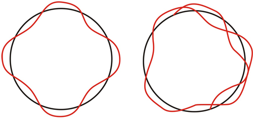
Figure 11: If a particle is constrained to move on a circle, its wave must resemble the left rather than the right drawing.
Source: © CK-12 Foundation
The quantum mechanical description of a particle is a mathematical function called a “wavefunction” related to the probability of finding the particle at any point in space. This function takes the form of a wave, hence the name wavefunction. If a particle is constrained to move in a circle, as it would be if it moves in a single, compactified dimension, the wave must oscillate some definite number of times around the circle as shown on the left side of the illustration above. The red line on the right side of the illustration does not correspond to a particle’s wavefunction because it doubles over on itself as it goes around the circle rather than coming back to the same point. Each possible number of oscillations around the circle corresponds to a distinct, or quantized, value of energy that the particle can have. We will learn more about quantum wavefunctions and quantized energy in Unit 5. (Unit: 4)
To understand precisely what elementary particles the 9D observer sees, we need to understand how the 10D particle is allowed to move on the circle. It turns out that this is quite simple. In quantum mechanics, as we will see in Units 5 and 6, the mathematical description of a particle is a “probability wave” that gives the likelihood of the particle being found at any position in space. The particle’s energy is related to the frequency of the wave: a higher frequency wave corresponds to a particle with higher energy. When the particle motion is confined to a circle, as it is for our particle moving in the compactified tenth dimension, the particle’s probability wave needs to oscillate some definite number of times (0, 1, 2 …) as one goes around the circle and comes back to the same point. Each possible number of oscillations on the circle corresponds to a distinct value of energy that the 10D particle can have, and each distinct value of energy will look like a new particle with a different mass to the 9D observer. The masses of these particles are related to the size of the circle, and the number of wave oscillations around the circle:
m0 = 0,m1 = 1/R,m2 = 2/R…
So, as promised, the hidden velocity in the tenth dimension gives rise to a whole tower of particles in nine dimensions.
Strings in a curled-up dimension
Now, let us consider a string theory compactified on the same circle as above. For all intents and purposes, if the string itself is not oscillating, it is just like the 10D particle we discussed above. The 9D experimentalist will see the single string give rise to an infinite tower of 9D particles with distinct masses. But that’s not the end of the story. We can also wind the string around the circular tenth dimension. To visualize this, imagine winding a rubber band around the thin part of a doorknob, which is also a circle. If the string has a tension Tstring = 1/ , (the conventional notation for the string tension), then winding the string once, twice, three times … around a circle of size R, costs an energy:
m1 = R/α‘,m3 = 2R /α‘m3 = 3R
This is because the tension is defined as the mass per unit length of the string; and if we wind the string n times around the circle, it has a length which is n times the circumference of the circle. Just as a 9D experimentalist cannot see momentum in the 10th dimension, she also cannot see this string’s winding number. Instead, she sees each of the winding states above as new elementary particles in the 9D world, with discrete masses that depend on the size of the compactified dimension and the string tension.
Geometry at short distances
One of the problems of quantum gravity raised in Section 2 is that we expect geometry at short distances to be different somehow. After working out what particles our 9D observer would expect to see, we are finally in a position to understand how geometry at short distances is different in a string theory.
The string tension, 1/α‘, is related to the length of the string, ℓstring, via α‘ = ℓstring2. Strings are expected to be tiny, with ℓstring ~ 10-32 centimeter, so the string tension is very high. If the circle is of moderate to macroscopic size, the winding modeparticles are incredibly massive since their mass is proportional to the size of the circle multiplied by the string tension. In this case, the 9D elementary particle masses in the string theory look much like that in the point particle theory on a circle of the same size, because such incredibly massive particles are difficult to see in experiments.

Figure 12: The consequences of strings winding around a larger extra dimension are the same as strings moving around a smaller extra dimension.
Strings in a compactified extra dimension can create lower-dimensional particles in two ways: by winding around the extra dimension, and by moving around the circle. It turns out that these are mathematically equivalent. Strings wound around a larger extra dimension, illustrated on the left, give rise to exactly the same set of particles as strings moving around a smaller extra dimension, shown on the right. This equivalence between large and small extends to the full string theory, and is an example of how string theories give rise to different short-distance physics than do particle theories, which is a critical feature of the theory of quantum gravity. (Unit: 4)
However, let us now imagine shrinking R until it approaches the scale of string theory or quantum gravity, and becomes less than ℓstring. Then, the pictures one sees in point particle theory, and in string theory, are completely different. When R is smaller than ℓstring, the modes m1, m2 … are becoming lighter and lighter. And at very small radii, they are low-energy excitations that one would see in experiments as light 9D particles.
In the string theory with a small, compactified dimension, then, there are two ways that a string can give rise to a tower of 9D particles: motion around the circle, as in the particle theory, and winding around the circle, which is unique to the string theory. We learn something very interesting about geometry in string theory when we compare the masses of particles in these two towers.
For example, in the “motion” tower, m1 = 1/R; and in the “winding” tower, m1 = R/α‘. If we had a circle of size /R instead of size R, we’d get exactly the same particles, with the roles of the momentum-carrying strings and the wound strings interchanged. Up to this interchange, strings on a very large space are identical (in terms of these light particles, at least) to strings on a very small space. This large/small equivalence extends beyond the simple considerations we have described here. Indeed, the full string theory on a circle of radius R is completely equivalent to the full string theory on a circle of radius α‘/R. This is a very simple illustration of what is sometimes called “quantum geometry” in string theory; string theories see geometric spaces of small size in a very different way than particle theories do. This is clearly an exciting realization because many of the mysteries of quantum gravity involve spacetime at short distances and high energies.
5. Extra Dimensions and Particle Physics
The Standard Model of particle physics described in Units 1 and 2 is very successful, but leaves a set of lingering questions. The list of forces, for instance, seems somewhat arbitrary: Why do we have gravity, electromagnetism, and the two nuclear forces instead of some other cocktail of forces? Could they all be different aspects of a single unified force that emerges at higher energy or shorter distance scales? And why do three copies of each of the types of matter particles exist—not just an electron but also a muon and a tau? Not just an up quark, but also a charm quark and a top quark? And how do we derive the charges and masses of this whole zoo of particles? We don’t know the answers yet, but one promising and wide class of theories posits that some or all of these mysteries are tied to the geometry or topology of extra spatial dimensions.
Perhaps the first attempt to explain properties of the fundamental interactions through extra dimensions was that of Theodor Kaluza and Oskar Klein. In 1926, soon after Einstein proposed his theory of general relativity, they realized that a unified theory of gravity and electromagnetism could exist in a world with 4+1 spacetime dimensions. The fifth dimension could be curled up on a circle of radius R so small that nobody had observed it.

Figure 13: Theodor Kaluza (left) and Oskar Klein (right) made a remarkable theoretical description of gravity in a fifth dimension.
Source: © Left: University of Göttingen, Right: Stanley Deser.
Theodor Kaluza (left) and Oskar Klein (right) conceived some of the most pervasive ideas in string theory today. Kaluza, a German mathematician and physicist, realized in 1919 that Maxwell’s equations of electricity and magnetism arise naturally from Einstein’s equations of general relativity if he added an extra dimension. Klein, a theoretical physicist in Sweden, realized in the 1920s that extra dimensions can be so small that we cannot observe them directly. While the theory known today as “Kaluza-Klein” gravity turned out not to describe the universe we live in, the novel ideas it contained are basic ingredients in nearly every modern string theory. (Unit: 4)
In the 5D world, there are only gravitons, the force carriers of the gravitational field. But, as we saw in the previous section, a single kind of particle in higher dimensions can give rise to many in the lower dimension. It turns out that the 5D graviton would give rise, after reduction to 4D on a circle, to a particle with very similar properties to the photon, in addition to a candidate 4D graviton. There would also be a whole tower of other particles, as in the previous section, but they would be quite massive if the circle is small, and can be ignored as particles that would not yet have been discovered by experiment.
This is a wonderful idea. However, as a unified theory, it is a failure. In addition to the photon, it predicts additional particles that have no counterpart in the known fundamental interactions. It also fails to account for the strong and weak nuclear forces, discovered well after Kaluza and Klein published their papers. Nevertheless, modern generalizations of this basic paradigm, with a few twists, can both account for the full set of fundamental interactions and give enormous masses to the unwanted additional particles, explaining their absence in low-energy experiments.
Particle generations and topology

Figure 1: Fundamental particles of the Standard Model.
One of the most obvious hints of substructure in the Standard Model is the presence of three generations of particles with the same quantum numbers under all the basic interactions. This is what gives the Standard Model the periodic table-like structure we saw in Unit 1. This kind of structure sometimes has a satisfying and elegant derivation in models based on extra dimensions coming from the geometry or topology of space itself. For instance, in string theories, the basic elementary particles arise as the lowest energy states, or ground states, of the fundamental string. The different possible string ground states, when six of the 10 dimensions are compactified, can be classified by their topology.
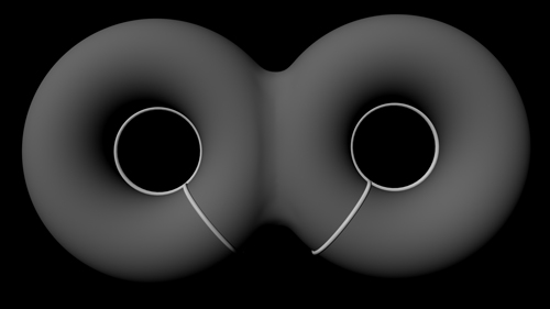
Because it is difficult for us to imagine six dimensions, we’ll think about a simpler example: two extra dimensions compactified on a two-dimensional surface. Mathematicians classified the possible topologies of such compact, smooth two-dimensional surfaces in the 19th century. The only possibilities are so-called “Riemann surfaces of genus g,” labeled by a single integer that counts the number of “holes” in the surface. Thus, a beach ball has a surface of genus 0; a donut’s surface has genus 1, as does a coffee mug’s; and one can obtain genus g surfaces by smoothly gluing together the surfaces of g donuts.

Figure 15: These objects are Riemann surfaces with genus 0, 1, and 2.
Source: © Left: Wikimedia Commons, Public Domain, Author: Norvy, 27 July 2006; Center: Wikimedia Commons, Public Domain, Author: Tijuana Brass, 14 December 2007; Right: Wikimedia Commons, Public Domain. Author, NickGorton, 22 August 2005
Riemann surfaces, named for the German mathematician Bernhard Riemann, who studied them, are classified by the number of holes they have. A ball has no holes, and is thus genus zero (g = 0), as is a drinking glass, a table, and any other object topologically equivalent to the ball. A coffee cup (with a handle) has one hole, and therefore has g = 1. An object with two holes, likewise, has g = 2. The six compactified dimensions of string theory form a Riemann surface. By studying the behavior of strings on Riemann surfaces with different values of g, theorists gain insight into how strings could generate the fundamental particles we have long observed in experiments. (Unit: 4)
To understand how topology is related to the classification of particles, let’s consider a toy model as we did in the previous section. Let’s think about a 6D string theory, in which two of the dimensions are compactified. To understand what particles a 4D observer will see, we can think about how to wind strings around the compactified extra dimensions. The answer depends on the topology of the two-dimensional surface. For instance, if it is a torus, we can wrap a string around the circular cross-section of the donut. We could also wind the string through the donut hole. In fact, arbitrary combinations of wrapping the hole N1 times and the cross-section N2 times live in distinct topological classes. Thus, in string theory on the torus, one obtains two basic stable “winding modes” that derive from wrapping the string in those two ways. These will give us two distinct classes of particles.

Figure 16: Strings can wind around a double torus in many distinct ways.
We have already seen how winding a string around an extra dimension gives rise to particles that can be observed from a lower dimensional space. Here, we have a g = 2 Riemann surface that looks like two donuts stuck together. A string can wind around the two different holes, and around the cross-section of each hole, giving four different winding modes. In general, a string has twice as many winding modes as there are holes in the Riemann surface to which the string is confined. Each mode corresponds to a class of particles, so the geometry of the extra dimensions has a clear physical consequence in the lower dimensional space. (Unit: 4)
Similarly, a Riemann surface of genus g would permit 2g different basic stable string states. In this way, one could explain the replication of states of one type—by, say, having all strings that wrap a circular cross-section in any of the g different handles share the same physical properties. Then, the replication of generations could be tied in a fundamental way to the topology of spacetime; there would, for example, be three such states in a genus 3 surface, mirroring the reality of the Standard Model.
Semi-realistic models of particle physics actually exist that derive the number of generations from specfic string compactifications on six-dimensional manifolds in a way that is very similar to our toy discussion in spirit. The mathematical details of real constructions are often considerably more involved. However, the basic theme—that one may explain some of the parameters of particle theory through topology—is certainly shared.
6. Extra Dimensions and the Hierarchy Problem

Figure 17: The weakness of gravity is difficult to maintain in a quantum mechanical theory, much as it is difficult to balance a pencil on its tip.
From a theoretical standpoint, the weakness of gravity relative to the other forces is unnatural. Maintaining this balance in a coherent mathematical framework is difficult, much as it is difficult to balance a pencil on its tip. Extra dimensions could help solve this hierarchy problem. (Unit: 4)
At least on macroscopic scales, we are already familiar with the fact that gravity, is 1040 times weaker than electromagnetism. We can trace the weakness of gravity to the large value of the Planck mass, or the smallness of Newton’s universal gravitational constant relative to the characteristic strength of weak interactions, which set the energy scale of modern-day particle physics. However, this is a description of the situation, rather than an explanation of why gravity is so weak.
This disparity of the scales of particle physics and gravity is known as the hierarchy problem. One of the main challenges in theoretical physics is to explain why the hierarchy problem is there, and how it is quantum mechanically stable. Experiments at the LHC should provide some important clues in this regard. On the theory side, extra dimensions may prove useful.
A speculative example
We’ll start by describing a speculative way in which we could obtain the vast ratio of scales encompassed by the hierarchy problem in the context of extra-dimensional theories. We describe this here not so much because it is thought of as a likely way in which the world works, but more because it is an extreme illustration of what is possible in theories with extra spatial dimensions. Let us imagine, as in string theory, that there are several extra dimensions. How large should these dimensions be?
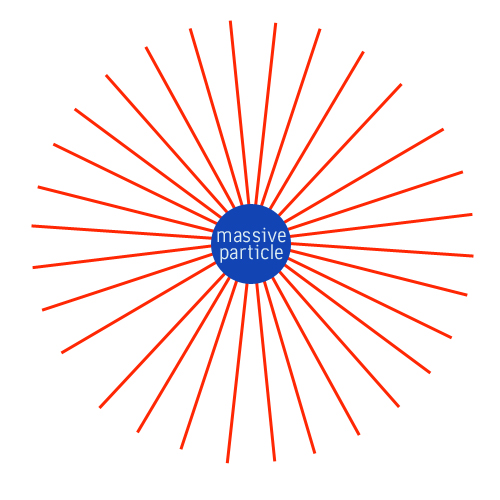
First, let us think a bit about a simple explanation for Newton’s law of gravitational attraction. A point mass in three spatial dimensions gives rise to a spherically symmetrical gravitational field: Lines of gravitational force emanate from the mass and spread out radially in all directions. At a given distance r from the mass, the area that these lines cross is the surface of a sphere of radius r, which grows like r2. Therefore, the density of field lines of the gravitational field, and hence the strength of the gravitational attraction, falls like 1/r2. This is the inverse square law from Unit 3.
Now, imagine there were k extra dimensions, each of size L. At a distance from the point mass that is small compared to L, the field lines of gravitation would still spread out as if they are in 3+k dimensional flat space. At a distance r, the field lines would cross the surface of a hypersphere of radius r, which grows like r2+k. Therefore the density of field lines and the strength of the field fall like 1/r2+k —more quickly than in three-dimensional space. However, at a distance large compared to L, the compact dimensions don’t matter—one can’t get a large distance by moving in a very small dimension—and the field lines again fall off in density like 1/r2. The extra-fast fall-off of the density of field lines between distance of order, the Planck length, and L has an important implication. The strength of gravity is diluted by this extra space that the field lines must thread.
An only slightly more sophisticated version of the argument above shows that with k extra dimensions of size L, one has a 3+1 dimensional Newton’s constant that scales like L-k. This means that gravity could be as strong as other forces with which we are familiar in the underlying higher-dimensional theory of the world, if the extra dimensions that we haven’t seen yet are large (in Planck units, of course; not in units of meters). Then, the relative weakness of gravity in the everyday world would be explained simply by the fact that gravity’s strength is diluted by the large volume of the extra dimensions, where it is also forced to spread.
The astute reader may have noticed a problem with the above explanation for the weakness of the gravitational force. Suppose all the known forces really live in a 4+k dimensional spacetime rather than the four observed dimensions. Then the field lines of other interactions, like electromagnetism, will be diluted just like gravity, and the observed disparity between the strength of gravity and electromagnetism in 4D will simply translate into such a disparity in 4+k dimensions. Thus, we need to explain why gravity is different.

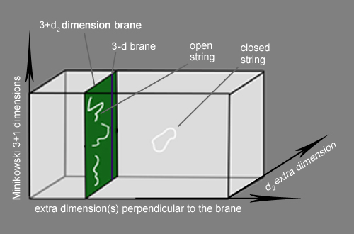
Figure 19: Strings can break open and end on a brane.
In addition to strings, string theories contain objects called “p-branes” that are essentially p-dimensional membranes on which strings can be confined. Strings can be closed loops that move around in the various dimensions, or they can break open and end on a p-brane. These open strings give rise to particles that only exist on the p-brane. It is possible that the world we live in is a 3-brane embedded in a higher dimensional space, and that the particles and forces we know are the product of open strings. (Unit: 4)
In string theories, a very elegant mechanism can confine all the interactions except gravity, which is universal and is tied directly to the geometry of spacetime, to just our four dimensions. This is because string theories have not only strings, but also branes. Derived from the term “membranes,” these act like dimensions on steroids. A p-brane is a p-dimensional surface that exists for all times. Thus, a string is a kind of 1-brane; for a 2-brane, you can imagine a sheet of paper extending in the x and y directions of space, and so on. In string theory, p-branes exist for various values of p as solutions of the 10D equations of motion.
So far, we have pictured strings as closed loops. However, strings can break open and end on a p-brane. The open strings that end in this manner give rise to a set of particles which live just on that p-brane. These particles are called “open string modes,” and correspond to the lowest energy excitations of the open string. In common models, this set of open string modes includes analogs of the photon. So, it is easy to get toy models of the electromagnetic force, and even the weak and strong forces, confined to a 3-brane or a higher dimensional p-brane in 10D spacetime.

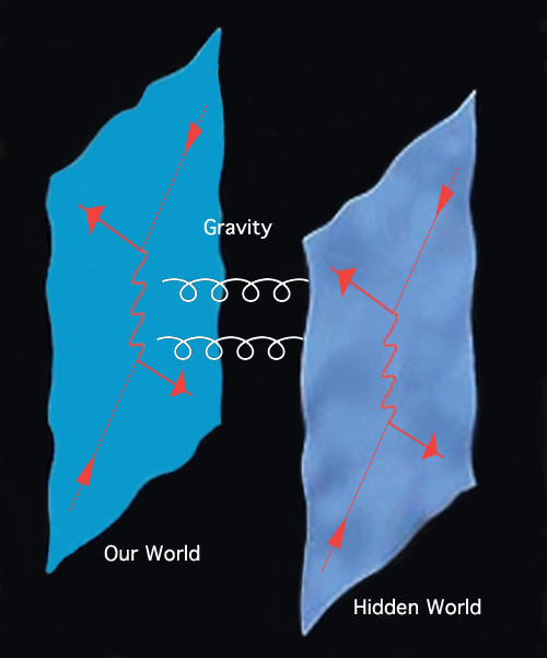
Figure 20: Gravity leaking into extra dimensions could explain the hierarchy problem.
One possible explanation of the hierarchy problem—why gravity is so much weaker than the other forces of nature—is that the force carriers of the strong, weak, and electromagnetic forces are confined to a three-dimensional brane on which we live, but the graviton is free to move in additional dimensions perpendicular to the brane. Hence, the gravitational force is diluted by the other dimensions while we perceive the other forces at full strength. (Unit: 4)
In a scenario that contains a large number of extra dimensions but confines the fundamental forces other than gravity on a 3-brane, only the strength of gravity is diluted by the other dimensions. In this case, the weakness of gravity could literally be due to the large unobserved volume in extra spacetime dimensions. Then the problem we envisioned at the end of the previous section would not occur: Gravitational field lines would dilute in the extra dimensions (thereby weakening our perception of gravity), while electromagnetic field lines would not.
While most semi-realistic models of particle physics derived from string theory work in an opposite limit, with the size of the extra dimensions close to the Planck scale and the natural string length scale around 10-32 centimeters, it is worth keeping these more extreme possibilities in mind. In any case, they serve as an illustration of how one can derive hierarchies in the strengths of interactions from the geometry of extra dimensions. Indeed, examples with milder consequences abound as explanations of some of the other mysterious ratios in Standard Model couplings.
7. The Cosmic Serpent
Throughout this unit, we have moved back and forth between two distinct aspects of physics: the very small (particle physics at the shortest distance scales) and the very large (cosmology at the largest observed distances in the universe). One of the peculiar facts about any modification of our theories of particle physics and gravity is that, although we have motivated them by thinking of short-distance physics or high-energy localized scattering, any change in short-distance physics also tends to produce profound changes in our picture of cosmology at the largest distance scales. We call this relationship between the very small and the very large the “cosmic serpent.”

Figure 21: Changes in short distance physics—at the Planck scale—can produce profound changes in cosmology, at the largest imaginable distances.
Theoretical physicists tend to use units of length, energy, and temperature interchangeably. Energy is related to temperature through the expression E = kT, where k is Boltzmann’s constant, so high energies correspond to high temperatures. Energy is proportional to 1/length, as we saw in section 2 and as we will see in a different context in Units 5 and 6. So, high energies and temperatures correspond to short distances. The scale in the diagram above is logarithmic, so each tick mark is separated by a factor of 100,000. It is amazing to realize that physics at the Planck scale is closely related to physics on cosmological scales nearly 60 orders of magnitude larger. (Unit: 4)
This connection has several different aspects. The most straightforward stems from the Big Bang about 13.7 billion years ago, which created a hot, dense gas of elementary particles, brought into equilibrium with each other by the fundamental interactions, at a temperature that was very likely in excess of the TeV scale (and in most theories, at far higher temperatures). In other words, in the earliest phases of cosmology, nature provided us with the most powerful accelerator yet known that attained energies and densities unheard of in terrestrial experiments. Thus, ascertaining the nature of, and decoding the detailed physics of, the Big Bang, is an exciting task for both particle physicists and cosmologists.
The cosmic microwave background
One very direct test of the Big Bang picture that yields a great deal of information about the early universe is the detection of the relic gas of radiation called the cosmic microwave background, or CMB. As the universe cooled after the Big Bang, protons and neutrons bound together to form atomic nuclei in a process called Big Bang nucleosynthesis, then electrons attached to the nuclei to form atoms in a process called . At this time, roughly 390,000 years after the Big Bang, the universe by and large became transparent to photons. Since the charged protons and electrons were suddenly bound in electrically neutral atoms, photons no longer had charged particles to scatter them from their path of motion. Therefore, any photons around at that time freely streamed along their paths from then until today, when we see them as the “surface of last scattering” in our cosmological experiments.
Bell Labs scientists Arno Penzias and Robert Wilson first detected the cosmic microwave background in 1964. Subsequent studies have shown that the detailed thermal properties of the gas of photons are largely consistent with those of a blackbody">recombination. At this time, roughly 390,000 years after the Big Bang, the universe by and large became transparent to photons. Since the charged protons and electrons were suddenly bound in electrically neutral atoms, photons no longer had charged particles to scatter them from their path of motion. Therefore, any photons around at that time freely streamed along their paths from then until today, when we see them as the “surface of last scattering” in our cosmological experiments.
Bell Labs scientists Arno Penzias and Robert Wilson first detected the cosmic microwave background in 1964. Subsequent studies have shown that the detailed thermal properties of the gas of photons are largely consistent with those of a blackbody at a temperature of 2.7 degrees Kelvin, as we will see in Unit 5. The temperature of the CMB has been measured to be quite uniform across the entire sky—wherever you look, the CMB temperature will not vary more than 0.0004 K.

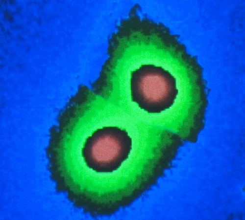
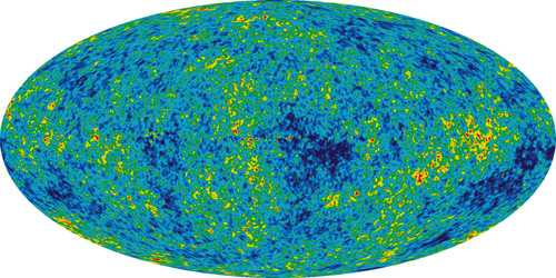
Figure 22: Map of the temperature variations in the cosmic microwave background measured by the WMAP satellite.
Source: © NASA, WMAP Science Team
This map shows the pattern of temperature variations in the cosmic microwave background (CMB) measured with the WMAP satellite. WMAP made a differential measurement of the CMB temperature with two sensitive radio antennae mounted with a fixed displacement between them. As the satellite rotated, the radio antennae traced out temperature variations in the entire sky. The largest temperature differences (between the red and dark blue regions) are about 0.0004 K, and the characteristic angular size of the temperature variations is around 1 degree. By analyzing the detailed pattern in this map, WMAP scientists infer that less than 4 percent of the universe is ordinary matter, and 23 percent is dark matter. (Unit: 4)
So, in the cosmic connection between particle physics and cosmology, assumptions about the temperature and interactions of the components of nuclei or atoms translate directly into epochs in cosmic history like nucleosynthesis or recombination, which experimentalists can then test indirectly or probe directly. This promising approach to testing fundamental theory via cosmological observations continues today, with dark matter, dark energy, and the nature of cosmic inflation as its main targets. We will learn more about dark matter in Unit 10 and dark energy in Unit 11. Here, we will attempt to understand inflation.
Cosmic inflation
Let us return to a puzzle that may have occurred to you in the previous section, when we discussed the gas of photons that started to stream through the universe 390,000 years after the Big Bang. Look up in the sky where you are sitting. Now, imagine your counterpart on the opposite side of the Earth doing the same. The microwave photons impinging on your eye and hers have only just reached Earth after their long journey from the surface of last scattering. And yet, the energy distribution (and hence the temperature) of the photons that you see precisely matches what she discovers.

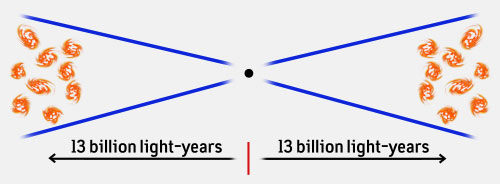
Figure 23: Both sides of the universe look the same, although light could not have traveled from one side to the other.
The universe appears to look the same in every direction, although the two opposite sides of the universe are far enough apart that light starting at one side traveling toward the other side could not have made it across in the time after the Big Bang. Normally when things look the same, it is because there is a causal connection between them, but that can’t be the case here. This is what physicists call the “horizon problem.” (Unit: 4)
How is this possible? Normally, for a gas to have similar properties (such as a common temperature) over a given distance, it must have had time for the constituent atoms to have scattered off of each other and to have transferred energy throughout its full volume. However, the microwave photons reaching you and your doppelgänger on the other side of the Earth have come from regions that do not seem to be in causal contact. No photon could have traveled from one to the other according to the naive cosmology that we are imagining. How then could those regions have been in thermal equilibrium? We call this cosmological mystery the “horizon problem.”
To grasp the scope of the problem, imagine that you travel billions of light-years into the past, find a distribution of different ovens with different manufacturers, power sources, and other features in the sky; and yet discover that all the ovens are at precisely the same temperature making Baked Alaska. Some causal process must have set up all the ovens and synchronized their temperatures and the ingredients they are cooking. In the case of ovens, we would of course implicate a chef. Cosmologists, who have no obvious room for a cosmic chef, have a more natural explanation: The causal structure of the universe differs from what we assume in our naive cosmology. We must believe that, although we see a universe expanding in a certain way today and can extrapolate that behavior into the past, something drastically different happened in the far enough past.

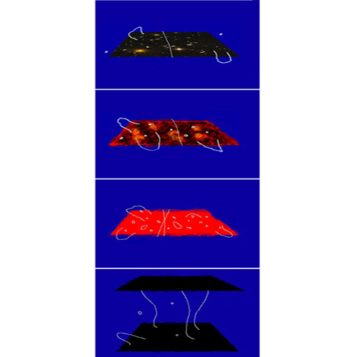
Figure 24: During the period of inflation, the universe grew by a factor of at least 1025.
Source: © NASA, WMAP Science Team
Inflation is the leading explanation for why our universe looks the same in every direction. If the universe expanded very rapidly, fluctuations and differences between different regions of space would have smoothed out. To explain what we observe in the cosmic microwave background, the universe must have expanded by at least a factor of 1025 in a tiny fraction of a second. (Unit: 4)
Cosmic inflation is our leading candidate for that something. Theories of cosmic inflation assert that the universe underwent a tremendously explosive expansion well before the last scattering of photons occurred. The expansion blew up a region of space a few orders of magnitude larger than the Planck scale into the size of a small grapefruit in just a few million Planck times (where a Planck time is 10-44seconds). During that brief period, the universe expanded by a factor of at least 1025. The inflation would thus spread particles originally in thermal contact in the tiny region a few orders of magnitude larger than the Planck length into a region large enough to be our surface of last scattering. In contrast, extrapolation of the post-Big Bang expansion of the universe into the past would never produce a region small enough for causal contact to be established at the surface of last scattering without violating some other cherished cosmological belief.
Inflation and slow-roll inflation
How does this inflation occur? In general relativity, inflation requires a source of energy density that does not move away as the universe expands. As we will see in Unit 11, simply adding a constant term (a cosmological constant) to Einstein’s equations will do the trick. But, the measured value of the present-day expansion rate means the cosmological constant could only have been a tiny, tiny fraction of the energy budget of the universe at the time of the Big Bang. Thus, it had nothing to do with this explosive expansion.

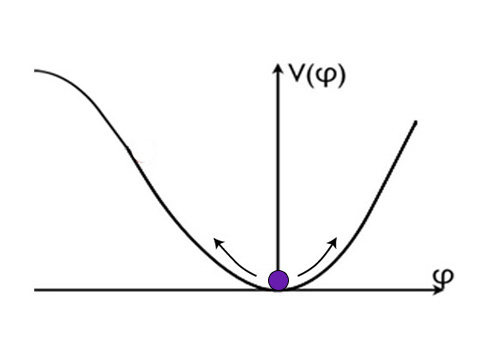
Figure 25: A potential like the one shown above for the inflaton field could have caused inflation.
The potential for the inflaton field shown above has a nearly flat region (upper left) slowly approaching a steeper slope that leads to an energy minimum. If started out in this flat region, evolving toward its minimum energy state, it would add a nearly constant amount to the energy density of the universe and inflation would proceed. (Unit: 4)
However, there could have been another source of constant energy density: not exactly a cosmological constant, but something that mimics one well for a brief period of a few million Planck times. This is possible if there is a new elementary particle, the inflaton, and an associated scalar field φ. The field φ evolves in time toward its lowest energy state. The energy of φ at any spacetime point is given by a function called its “potential.” If φ happens to be created in a region where the potential varies extremely slowly, then inflation will proceed. This is quite intuitive; the scalar field living on a very flat region in its potential just adds an approximate constant to the energy density of the universe, mimicking a cosmological constant but with a much larger value of the energy density than today’s dark energy. We know that a cosmological constant causes accelerated (in fact, exponential) expansion of the universe.
As inflation happens,  will slowly roll in its potential as the universe exponentially expands. Eventually, reaches a region of the potential where this peculiar flatness no longer holds configuration. As it reaches the ground state, its oscillations result in the production of the Standard Model quarks and leptons through weak interactions that couple them to the inflaton. This end of inflation, when the energy stored in the inflation field is dumped into quarks and leptons, is what we know as the Big Bang.

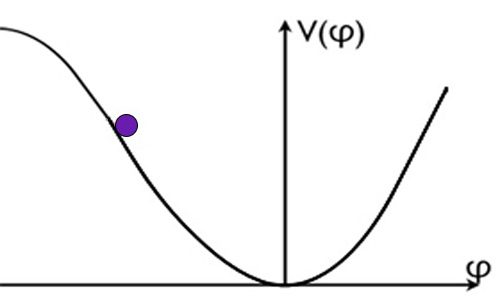
Figure 26: All the Standard Model particles could have been produced by the inflaton oscillating around its ground state like a ball rolling around in a valley.
If the inflaton model of inflation is correct, then the universe stops expanding as the inflaton field rolls down the steep slope in its potential. When it reaches the bottom of this hill, the field oscillates around the minimum. As we have learned in Unit 2, the oscillations of fundamental fields give rise to particles. So the oscillating of the inflaton field could create all the matter we see in the universe, and the end of inflation could be what we call the Big Bang. (Unit: 4)
We can imagine how this works by thinking about a ball rolling slowly on a very flat, broad hilltop. The period of inflation occurs while the ball is meandering along the top. It ends when the ball reaches the edge of the hilltop and starts down the steep portion of the hill. When the ball reaches the valley at the bottom of the hill, it oscillates there for a while, dissipating its remaining energy. However, the classical dynamics of the ball and the voyage of the inflaton differ in at least three important ways. The inflaton’s energy density is a constant; it suffuses all of space, as if the universe were filled with balls on hills (and the number of the balls would grow as the universe expands). Because of this, the inflaton sources an exponentially fast expansion of the universe as a whole. Finally, the inflaton lives in a quantum world, and quantum fluctuations during inflation have very important consequences that we will explore in the next section.
8. Inflation and the Origin of Structure

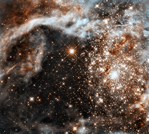
Figure 27: While the universe appears approximately uniform, we see varied and beautiful structure on smaller scales.
Source: © NASA, ESA, and F. Paresce (INAPF-AIASF, Bologna, Italy).
It is a basic tenet of cosmology that the universe is homogeneous and isotropic, which means that it looks basically the same in all directions. However, as this Hubble Space Telescope image (actually a combination of two images taken at different wavelengths) shows, there is a wide variety of small-scale structure in the universe. Here, we see a star-forming region in a satellite galaxy of the Milky Way. This image contains some of the most massive known stars and coalescing gas clouds in a young stellar grouping called “R136.” (Unit: 4)
On the largest cosmological scales, the universe appears to be approximately homogeneous and isotropic. That is, it looks approximately the same in all directions. On smaller scales, however, we see planets, stars, galaxies, clusters of galaxies, superclusters, and so forth. Where did all of this structure come from, if the universe was once a smooth distribution of hot gas with a fixed temperature?
The temperature of the fireball that emerged from the Big Bang must have fluctuated very slightly at different points in space (although far from enough to solve the horizon problem). These tiny fluctuations in the temperature and density of the hot gas from the Big Bang eventually turned into regions of a slight overdensity of mass and energy. Since gravity is attractive, the overdense regions collapsed after an unimaginably long time to form the galaxies, stars, and planets we know today. The dynamics of the baryons, dark matter, and photons all played important and distinct roles in this beautiful, involved process of forming structure. Yet, the important point is that, over eons, gravity amplified initially tiny density fluctuations to produce the clumpy astrophysics of the modern era. From where did these tiny density fluctuations originate? In inflationary theory, the hot gas of the Big Bang arises from the oscillations and decay of the inflaton field itself. Therefore, one must find a source of slight fluctuations or differences in the inflaton’s trajectory to its minimum, at different points in space. In our analogy with the ball on the hill, remember that inflation works like a different ball rolling down an identically shaped hill at each point in space. Now, we are saying that the ball must have chosen very slightly different trajectories at different points in space—that is, rolled down the hill in very slightly different ways.

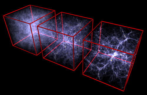
Figure 28: Small fluctuations in density in the far left box collapse into large structures on the right in this computer simulation of the universe.
Source: © Courtesy of V. Springel, Max-Planck-Institute for Astrophysics, Germany.
One source of fluctuations is quantum mechanics itself. The roll of the inflaton down its potential hill cannot be the same at all points in space, because small quantum fluctuations will cause tiny differences in the inflaton trajectories at distinct points. But because the inflaton’s potential energy dominates the energy density of the universe during inflation, these tiny differences in trajectory will translate to small differences in local energy densities. When the inflaton decays, the different regions will then reheat the Standard Model particles to slightly different temperatures.
Who caused the inflation?
This leaves our present-day understanding of inflation with the feel of a murder mystery. We’ve found the body—decisive evidence for what has happened through the nearly uniform CMB radiation and numerous other sources. We have an overall framework for what must have caused the events, but we don’t know precisely which suspect is guilty; at our present level of knowledge, many candidates had opportunity and were equally well motivated.

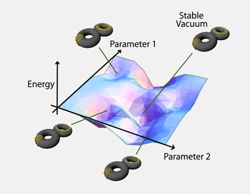
Figure 29: Typical string theories or supersymmetric field theories have many candidate scalar field inflatons.
The goal of inflationary theory is to determine the inflaton that was responsible for expanding the patch of the universe we can observe. It’s possible that different scalar fields inflated different patches of the universe. Typical string or supersymmetric field theories have many candidate scalar field inflatons that parameterize the shape of the extra dimensions. (Unit: 4)
In inflationary theory, we try to develop a watertight case to convict the single inflaton that was relevant for our cosmological patch. However, the suspect list is a long one, and grows every day. Theories of inflation simply require a scalar field with a suitable potential and some good motivation for the existence of that scalar and some rigorous derivation of that potential. At a more refined level, perhaps they should also explain why the initial conditions for the field were just right to engender the explosive inflationary expansion. Modern supersymmetric theories of particle physics, and their more complete embeddings into unified frameworks like string theory, typically provide abundant scalar fields.
While inflationary expansion is simple to explain, it is not simple to derive the theories that produce it. In particular, inflation involves the interplay of a scalar field’s energy density with the gravitational field. When one says one wishes for the potential to be flat, or for the region over which it is flat to be large, the mathematical version of those statements involves MPlanck in a crucial way: Both criteria depend on MPlanck2 multiplied by a function of the potential. Normally, we don’t need to worry so much about terms in the potential divided by powers of MPlanck because the Planck mass is so large that these terms will be small enough to neglect. However, this is no longer true if we multiply by MPlanck2. Without going into mathematical details, one can see then that even terms in the potential energy suppressed by a few powers of MPlanck can qualitatively change inflation, or even destroy it. In the analogy with the rolling ball on the hill, it is as if we need to make sure that the hilltop is perfectly flat with well-mown grass, and with no gophers or field mice to perturb its flat perfection with minute tunnels or hills, if the ball is to follow the inflation-causing trajectory on the hill that we need it to follow.

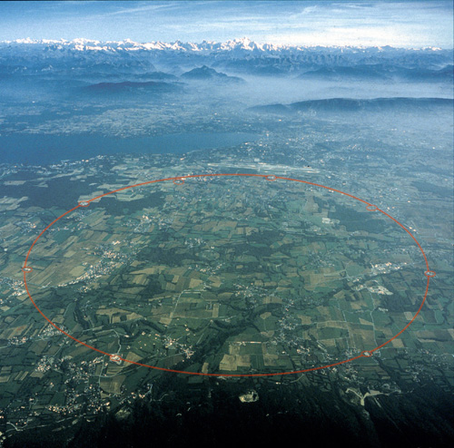
Figure 30: The LHC creates the highest-energy collisions on Earth, but these are irrelevant to Planck-scale physics.
Source: © CERN.
The Large Hadron Collider (LHC), shown here from above, is capable of creating the highest-energy collisions on Earth, with a center-of-mass energy of 14 TeV. Unfortunately, even the LHC does not come close to measuring the Planck-scale physics that was important for inflation. To learn about those, we must rely on observational cosmology to find clues to what happened in the largest particle accelerator of all: the Big Bang. (Unit: 4)
In particle physics we will probe the physics of the TeV scale at the LHC. There, we will be just barely sensitive to a few terms in the potential suppressed by a few TeV. Terms in the potential that are suppressed by MPlanck are, for the most part, completely irrelevant in particle physics at the TeV scale. If we use the cosmic accelerator provided by the Big Bang, in contrast, we get from inflation a predictive class of theories that are crucially sensitive to quantum gravity or string theory corrections to the dynamics. This is, of course, because cosmic inflation involves the delicate interplay of the inflaton with the gravitational field.
9. Inflation in String Theory
Because inflation is sensitive to MPlanck-suppressed corrections, physicists must either make strong assumptions about Planck-scale physics or propose and compute with models of inflation in theories where they can calculate such gravity effects. String theory provides one class of theories of quantum gravity well developed enough to offer concrete and testable models of inflation—and sometimes additional correlated observational consequences. A string compactification from 10D to 4D often introduces interesting scalar fields. Some of those fields provide intriguing inflationary candidates.

Figure 31: A brane and an anti-brane moving toward one another and colliding could have caused inflation and the Big Bang.
Source: © S.-H. Henry Tye Laboratory at Cornell University. More info
An intriguing possible explanation for inflation is the attraction of a brane and an antibrane. The brane-antibrane attraction is similar to the attraction between an electron and its antiparticle, the positron. When the two branes are far apart, they move toward one another slowly, producing slow-roll inflation. When they get close enough together, they accelerate into each other and slam together in a collision that could have produced all the matter in the universe today. (Unit: 4)
Perhaps the best-studied classes of models involve p-branes of the sort we described earlier in this unit. So just for concreteness, we will briefly describe this class of models. Imagine the cosmology of a universe that involves string theory compactification, curling up six of the extra dimensions to yield a 4D world. Just as we believe that the hot gas of the Big Bang in the earliest times contained particles and anti-particles, we also believe that both branes and anti-branes may have existed in a string setting; both are p-dimensional hyperplanes on which strings can end, but they carry opposite charges under some higher-dimensional analog of electromagnetism.
The most easily visualized case involves a 3-brane and an anti-3-brane filling our 4D spacetime but located at different points in the other six dimensions. Just as an electron and a positron attract one another, the brane and anti-brane attract one another via gravitational forces as well as the other force under which they are charged. However, the force law is not exactly a familiar one. In the simplest case, the force falls off as 1/r4, where r is the distance separating the brane and anti-brane in the 6D compactified space.
Models with sufficiently interesting geometries for the compactified dimensions can produce slow-roll inflation when the brane and anti-brane slowly fall together, under the influence of the attractive force. The inflaton field is the mode that controls the separation between the brane and the anti-brane. Each of the branes, as a material object filling our 4D space, has a tension that provides an energy density filling all of space. So, a more accurate expression for the inter-brane potential would be V(r) ~ 2T3 − 1/r4, where T3 is the brane tension. For sufficiently large r and slowly rolling branes, the term 2T3 dominates the energy density of the universe and serves as the effective cosmological constant that drives inflation.
As the branes approach each other and r ~ ℓstring, this picture breaks down. This is because certain open strings, now with one end on each of the branes as opposed to both ends on a single brane, can become light. In contrast, when r >> ℓstring, such open strings must stretch a long distance and are quite heavy. Remember that the energy or mass of a string scales with its length. In the regime where r is very small, and the open strings become light, the picture in terms of moving branes breaks down. Instead, some of the light open strings mediate an instability of the brane configuration. In the crudest approximation, the brane and anti-brane simply annihilate (just as an electron and anti-electron would), releasing all of the energy density stored in the brane tensions in the form of closed-string radiation. In this type of model, the Big Bang is related to the annihilation of a brane with an anti-brane in the early universe.
Other consequences of inflation
Any well-specified model of cosmic inflation has a full list of consequences that can include observables beyond just the density fluctuations in the microwave background that result from inflation. Here, we mention some of the most spectacular possible consequences.
Quantum jiggles: We do not know the energy scale of inflation directly from data. In many of the simplest theories, however, this energy scale is very high, close to the Grand Unified Theory scale of 1016 GeV. It is therefore quite possible that inflation is probing energies 13 orders of magnitude higher than we’ll see at the LHC.

Figure 32: A cosmic string could produce a double image of a galaxy behind it.
Source: © NASA/ESA Hubble Space Telescope. More info
The brane annihilation that ends inflation in the brane inflation model could produce giant strings that stretch across the entire universe. These cosmic strings are very massive because a string’s mass scales with its length. If the cosmic string happened to pass between us and a background galaxy, we would see a double image of the galaxy produced by the gravitational lensing process explained in Units 3 and 10. The signature of cosmic string lensing is the discontinuous break between the two galaxies in the simulated data shown here. (Unit: 4)
If the scale of inflation is high enough, we may see further corroborating evidence beyond the solution of the horizon problem and the explanation of density fluctuations. The density fluctuations we discussed in the previous section came from the quantum jiggles of the inflaton field itself. But during inflation, quantum jiggles also originate in the other fields present, including the gravitational field. Future cosmological experiments exploring those phenomena could pin down the scale of inflation to just a few orders of magnitude shy of the Planck scale.
Cosmic strings: Very particular models often come with their own smoking-gun signatures. Take, for example, the class of speculative models we discussed earlier based on the slow attraction and eventual annihilation of a 3-brane and an anti-3-brane. The annihilation process involves the dynamics of open strings that stretch between the 3-brane and its partner, and that eventually “condense.” This condensation process creates cosmic strings as the branes annihilate, which can be thought of as 1-branes or even fundamental strings that thread our 4D spacetime, and have grown to macroscopic size. If these tension-bearing cosmic strings really were created at the end of inflation, they should be present in the universe today, with tell-tale signatures in experiments that study the distribution of matter through gravitational lensing. Future experiments should rule out the presence of such strings or detect them for a wide range of values of the possible scale of inflation.

Figure 33: The Planck satellite will make precise measurements of fluctuations in the CMB.
Source: © ESA
The Planck mission, using a satellite launched by the European Space Agency in 2009, is to survey the cosmic microwave background with ten times more sensitivity and three times the resolution of the previous measurement. The fine-grained CMB map it produces may contain the detail required to divine the nature of inflation. (Unit: 4)
Density fluctuations: The slow-roll approach to inflation, with an inflaton field moving on a flat potential, is the class of models we focused on in the last section, but is not the only model of inflation. In some more modern theories, again partially inspired by branes in superstring theory, the inflaton undergoes rapid motion. Instead of the flatness of the potential, a delicate interplay between the potential and the complicated structure of the inflation kinetic terms produces the inflation. If any such model captures a grain of truth, then the pattern of density fluctuations would bear tell-tale structural signatures. Measurements by the Planck satellite that the European Space Agency launched in May 2009 should put constraints on the validity of those models.
10. Fundamental Questions of Gravity

Figure 34: Some of Einstein’s great insights began in thought experiments.
Source: © Marcelo Gleiser
While string theory has not yet directly confronted experiment, it is important to remember that some of the most influential ideas in modern physics have their roots in pure thought experiments. Einstein is perhaps the most famous thought experimentalist, conceiving the theory of relativity by working through a series of clever hypothetical scenarios. (Unit: 4)
Quantum gravity is not a mystery that is, as yet, open to experiment. With a few exceptions such as inflationary cosmology and, quite possibly, the correct interpretation of dark energy (see Unit 11), thoughts about quantum gravity remain in the theoretical realm. This does not mean that theories of quantum gravity cannot be important and testable in some circumstances. In a given model, for instance, string theory models of particle physics make very definite statements about the origins of the mass hierarchy of fermions or the number of generations of Standard Model particles. But these problems may also have other solutions, insensitive to the structure of gravity at short distances; only in very few cases do we suspect that quantum gravity must be a part of the solution to a problem.
Here, we discuss some of these issues that are intrinsically gravitational. They have not yet confronted experiment directly. But we should remember that Einstein formulated special relativity by reconciling different thought experiments, and that therefore even thought experiments about quantum gravity may eventually be useful.
Black holes and entropy
Black holes are objects so dense that the escape velocity from their surface exceeds the speed of light, c. Because of that, one would think that in a relativistic theory, outside observers performing classical experiments can never see their surfaces. As a rough-and-ready definition, we will call the surface defining the region where light itself can no longer escape from the gravitational attraction of a black hole, the event horizon. Nothing, in a classical theory, can be emitted from this horizon, though many things can fall through.

Figure 35: Artist’s conception of a black hole accreting matter from a companion star.
Source: © Dana Berry (CfA, NASA).
Black holes like the one illustrated here are thought to accumulate matter by pulling it off nearby objects with their strong gravitational interaction. When a black hole accretes matter, its energy grows with its mass, and its entropy grows with its surface area. (Unit: 4)
Careful consideration of the theory of black holes in classical general relativity in the early 1970s led Jacob Bekenstein, Stephen Hawking, and others to a striking set of conclusions. They found that as a chargeless, non-rotating black hole accretes matter, its mass grows by an amount proportional to the strength of gravity at the black hole’s surface and the change in its surface area. Also, the black hole’s surface area (defined by its event horizon) cannot decrease under any circumstances, and usually increases in time.
At a heuristic level, Bekenstein and Hawking’s laws for black holes seem reminiscent of the laws of thermodynamics and statistical mechanics: The change in energy is proportional to the change in entropy and the entropy (a measure of disorder) of a system can only increase. This is no coincidence. The results of general relativity imply what they seem to: A black hole does carry an entropy proportional to its surface area, and, of course, it has an energy that grows with its mass.

Figure 36: Black holes radiate by a quantum mechanical process.
Source: © Reprinted with permission from Nova Science Publishers, Inc. from: Sabine Hossenfelder, “What Black Holes Can Teach Us,” in Focus on Black Hole Research, ed. Paul V. Kreitler (New York: Nova Publishers Inc., 2006), 121-58.
Black holes are objects so massive that gravity prevents matter from escaping them. But black holes are warm or even hot, and we will see in Unit 5 that hot bodies radiate. How is it possible for anything to escape a black hole? The answer, as Stephen Hawking insightfully showed, is quantum mechanics. Black holes can emit photons and other particles, now known as “Hawking radiation,” through a quantum process that general relativity cannot explain. (Unit: 4)
One mystery remains, however. In thermodynamics, the change in energy is proportional to the temperature times the change in entropy; and hot bodies radiate. Even though there is an analogous quantity—the surface gravity—in the black hole mechanics, no classical process can bring radiation through the horizon of a black hole. In a brilliant calculation in 1974, Stephen Hawking showed that, nevertheless, black holes radiate by a quantum process. This quantum effect occurs at just the right level to make the analogy between black hole thermodynamics and normal thermodynamics work perfectly.
Hawking’s calculation reinforces our belief that a black hole’s entropy should be proportional to its surface area. This is a bit confusing because most theories that govern the interactions of matter and force-carrying particles in the absence of gravity posit that entropy grows in proportion to the volume of the system. But in a gravity theory also containing these other degrees of freedom, if one tries to fill a region with enough particles so that their entropy exceeds the area bounding the region, one instead finds gravitational collapse into a black hole, whose entropy is proportional to its surface area. This means that at least in gravity theories, our naive idea that the entropy that can be contained in a space should scale with its volume must be incorrect.
Holography, multiple dimensions, and beyond
This concept that in every theory of quantum gravity, the full entropy is proportional only to the area of some suitably chosen boundary or “holographic screen” in the system, and not the full volume, carries a further implication: that we may be able to formulate a theory of gravity in D +1 spacetime dimensions in just D dimensions—but in terms of a purely non-gravitational quantum field theory. Dutch theorist Gerard ‘t Hooft and his American colleague Leonard Susskind put forward this loose idea, called holography, in the early 1990s. The idea, as stated, is a bit vague. It begs questions such as: On which “bounding surface” do we try to formulate the physics? Which quantum field theory is used to capture which quantum gravity theory in the “bulk” of the volume?
In the late 1990s, through the work of Argentine theorist Juan Maldacena and many others, this idea received its first very concrete realization. We will focus on the case of gravity in four dimensions; for different reasons, much of the actual research has been focused on theories of gravity in five dimensions. This work gives, for the first time, a concrete non-perturbative formulation of quantum gravity in the 4D Anti de Sitter spacetime—the simplest solution of Einstein’s theory with a negative cosmological constant.

Figure 37: The AdS/CFT duality relates a theory on the boundary of a region to a theory with gravity in the interior.
It turns out that the symmetries of the 4D space—that is, in 3+1 dimensions—match those of a quantum field theory of a very particular sort, called a “conformal field theory,” in 2+1 spacetime dimensions. However, we also expect that quantum gravity in 3+1 dimensions should have the same behavior of its thermodynamic quantities (and in particular, its entropy) as a theory in 2+1 dimensions, without gravity. In fact, these two observations coincide in a beautiful story called the Anti de Sitter/Conformal Field Theory (AdS/CFT) correspondence. Certain classes of quantum field theories in 2+1 dimensions are exactly equivalent to quantum gravity theories in 3+1 dimensional Anti de Sitter space. Physicists say that these two theories are dual to one another.
The precise examples of this duality that we recognize come from string theory. Compactifications of the theory to four dimensions on different compact spaces give rise to different examples of AdS4 gravity and to different dual field theories. While we do not yet know the gravity dual of every 2+1 dimensional conformal field theory or the field theory dual of every gravity theory in AdS4, we do have an infinite set of explicit examples derived from string theory.
The value of duality
This duality has a particularly interesting, useful, and, on reflection, necessary aspect. The 2+1 dimensional field theories analogous to electromagnetism have coupling constants g analogous to the electron charge e. The gravity theory also has a natural coupling constant, given by the ratio of the curvature radius of space to the Planck length, which we will call L. In the known examples of the duality between AdS space and quantum field theories, large values of L, for which the gravity theory is weakly curved, and hence involves only weak gravity, correspond to very large values of g for the quantum field theory. Conversely, when the quantum field theory is weakly coupled (at small values of g), the gravity theory has very small L; it is strongly coupled in the sense that quantum gravity corrections (which are very hard to compute, even in string theory) are important.
This kind of duality, between a strongly coupled theory on the one hand and a weakly coupled theory on the other, is actually a common (though remarkable and beautiful) feature in physical theories. The extra shock here is that one of the theories involves quantum gravity in a different dimension.
This duality has had two kinds of uses to date. One obvious use is that it provides a definition of quantum gravity in terms of a normal field theory for certain kinds of gravitational backgrounds. Another use, however, that has so far proved more fruitful, is that it gives a practical way to compute in classes of strongly coupled quantum field theories: You can use their weakly curved gravitational dual and compute the dual quantities in the gravity theory there.

Figure 38: The aftermath of a heavy ion collision at RHIC, the Relativistic Heavy Ion Collider.
Source: © Courtesy of Brookhaven National Laboratory.
The aftermath of a high-energy collision between heavy ions, such as the one shown here, is an exotic state of matter called a “quark-gluon plasma.” The particles in the plasma are strongly interacting, so it is thus difficult to understand their behavior using conventional methods of calculation. The AdS/CFT duality, which links two separate theoretical descriptions of the same physics, has been used to model the outcome of collisions in the Relativistic Heavy Ion Collider at Brookhaven and has successfully predicted certain properties of the plasma, including the tiny ratio of its viscosity to its entropy. (Unit: 4)
Physicists have high hopes that such explorations of very strongly coupled quantum field theories based on gravity duals may provide insight into many of the central problems in strongly coupled quantum field theory; these include a proper understanding of quark confinement in QCD, the ability to compute transport in the strongly coupled QCD plasma created at present-day accelerators like Brookhaven National Laboratory’s Relativistic Heavy Ion Collider (RHIC) that smash together heavy ions, the ability to solve for quantities such as conductivity in strongly correlated electron systems in condensed matter physics, and an understanding of numerous zero-temperature quantum phase transitions in such systems. However, we must note that, while this new approach is orthogonal to old ones and promises to shed new light in various toy models of those systems, it has not yet helped to solve any of the central problems in those subjects.
The initial singularity
Even more intriguing is the question of the initial cosmological singularity. In general relativity, one can prove powerful theorems showing that any expanding cosmology (of the sort we inhabit) must have arisen in the distant past from a point of singularity in which the energy density and curvature are very large and the classical theory of relativity is expected to break down. Intuitively, one should just run the cosmological expansion backwards; then the matter we currently see flying apart would grow into an ever-denser and more highly curved state.

Figure 39: If we run time backwards, the entire universe collapses into a single, infinitely dense point.
Source: © NASA, WMAP Science Team.
The success of our standard model of cosmology in explaining phenomena observed in the universe today gives us confidence to extrapolate back in time to when the temperature of the universe was a few MeV. The Big Bang clearly happened before that, at TeV temperatures, but we do not know how it took place. Was there really an initial singularity, in which all the energy in the universe today was packed into a single point? How could the singularity itself have appeared? These remain open questions, at the forefront of modern gravitational research. (Unit: 4)
Our current picture of the Big Bang, including the successes of Big Bang nucleosynthesis and the CMB, gives us confidence that we can safely extrapolate our current cosmology back to temperatures of order MeV. In most inflationary theories, the Big Bang engendered temperatures far above the TeV scale. But at some still higher energy scale, probing the start of inflation and beyond, we do not know what happened; we do not even have any ideas that provide hints of testable predictions.
What is the origin of our observable universe? Is it one of many, coming from quantum tunneling events out of regions of space with different macroscopic laws of physics? Or is it a unique state, arising from some unknown initial condition of quantum gravity that we have yet to unravel? And, how does this physics eventually deal with the singularity theorems of general relativity, which assure us that extrapolation backwards into the past will lead to a state of high density and curvature, where little can be reliably calculated? These mysteries remain at the forefront of modern research in quantum gravity.
11. Further Reading
- Brian Greene, “The Elegant Universe,” Vintage Books, 2000.
- Juan Maldacena, “The Illusion of Gravity,” Scientific American, November, 2005, p. 56–63.
- Lisa Randall, “Warped Passages: Unraveling Mysteries of the Universe’s Hidden Dimensions,” Harper Perennial, 2006.
- Barton Zwiebach, “A First Course in String Theory,” Cambridge University Press, 2009.
The Math
Planck length and Planck mass
We can use dimensional analysis to construct a length and a mass scale using Planck’s constant, ℏ , Newton’s universal gravitational constant, G, and the speed of light, c.
Planck’s constant has units of: length2  mass
mass  time
time
Newton’s constant has units of: length3 (mass time2)
The speed of light has units of: length/time
We can construct a new constant that has units of length as follows:

The above expression has units of:

If we instead combine ℏ , G, and c into a new constant with units of mass, we find:

When we plug in actual numbers, we find that the Planck length is 1.61 x 10⁻³⁵ m, 1020 times smaller than the nucleus of an atom. The Planck mass (which, of course, also determines an energy scale) is around 10-5 g, which is equivalent to ~ 1019 GeV. These length and mass scales help physicists estimate when it’s necessary to do a calculation using a quantum theory of gravity.
Potential Energy and Force
The potential energy between two bound quarks grows linearly with the distance between the quarks:
V(x) ∝ Tstring x
V(x) is the potential energy, which is a function of the distance, x, between the quarks. The force between the quarks is proportional to the derivative (rate of change) of the potential:
F(x) ∝ dV(x)/dx ∝ Tstring
Therefore, the strong force between two quarks stays constant as the quarks are pulled apart.